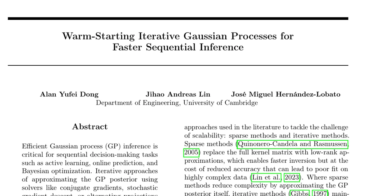
Warm-Starting Iterative Gaussian Processes for Faster Sequential Inference

AI summary

Overview

Research area: Machine learning — scalable Gaussian process inference, iterative linear solvers, sequential decision-making (Bayesian optimization, active learning, online prediction).

Technical level: Advanced. The paper assumes familiarity with Gaussian processes, covariance matrices, quadratic objectives, and iterative solvers, and it includes derivations in reproducing kernel Hilbert space (RKHS) norms.

Scope: This paper proposes and evaluates three warm-start initialization strategies that reuse the solution of a previously solved, smaller linear system to accelerate iterative GP posterior updates in sequential settings, with theory, regression benchmarks, and a parallel Thompson sampling study.

What This Paper Is About

Gaussian process posteriors require solving a linear system whose size grows each time new data arrive, and iterative solvers such as conjugate gradients (CG), stochastic gradient descent (SGD), or alternating projections (AP) avoid cubic cost but need many iterations when started from zero. The authors ask whether the solution of the previous, smaller system can be reused to initialize the larger extended system, so that fewer iterations are needed and the posterior update becomes cheaper without sacrificing accuracy. Their goal is to speed up sequential GP inference at a fixed tolerance, and to produce more accurate posteriors at a fixed compute budget.

Key Contributions

1. Three warm-start initializations for the extended linear system. The naïve warm-start keeps the previous weights for the original data points and sets the new weights to zero (cost O(1)); the residual line search sets the new weights to a scalar multiple of the residual, with the optimal step derived as α* = (rᵀr)/(rᵀH₂₂r) (cost O(n₂²)); and the marginal system solve sets the new weights to H₂₂⁻¹r, the value minimizing the quadratic objective given the fixed old weights (cost O(n₂³)).

2. Theoretical analysis of the initial RKHS distance. The authors show that the squared RKHS distance from the initialization to the exact solution satisfies d²_cold − d²_naïve = b₁ᵀH₁₁⁻¹b₁ ≥ 0, that d²_naïve − d²_line-search = (rᵀr)²/(rᵀH₂₂r) > 0, that d²_naïve − d²_marginal-solve = rᵀH₂₂⁻¹r > 0, and that the marginal system solve dominates the line search since rᵀH₂₂⁻¹r ≥ (rᵀr)²/(rᵀH₂₂r). They further connect reducing this RKHS distance to optimizing the quadratic objective and to reducing the residual used as the solver stopping criterion.

3. Regression benchmarks on real-world datasets. Across 3droad (3drd), pol, protein (prot), bike, and buzz, when solving to tolerance τ = 0.01, the methods reduce solver iterations and produce speed-ups.

4. Parallel Thompson sampling experiments under a fixed compute budget. With capped solver iterations, warm-starting yields smaller final residuals, more accurate posteriors, and better optimization performance.

Main Findings

• Large speed-ups when solving to tolerance: Warm-starting achieves speed-ups of up to 2.2× for SGD, 1.8× for CG, and 19.2× for AP. The abstract summarizes this as "speed-ups of up to 19× when solving to tolerance."

• Average iteration reductions (posterior mean and sample systems combined): The naïve method reduces solver iterations by approximately 30% for CG, 34% for SGD, and 75% for AP, equivalent to 1.4×, 1.5×, and 4.0× speed-ups. The reduction for AP reaches up to 94.6% on some datasets, equivalent to a 19× speed-up.

• Residual line search averages: 25%, 37%, and 76% iteration reductions, or 1.3×, 1.6×, and 4.2× speed-ups for CG, SGD, and AP.

• Marginal system solve averages: 33%, 41%, and 76% iteration reductions, or 1.5×, 1.7×, and 4.2× speed-ups for CG, SGD, and AP.

• Initial distance reductions (regression, 1000 initial + 100 new data points): The naïve method places initial weights roughly 70% closer to the final solution on average than cold-starting, for all datasets. Setting values for the new weights gives a further average 4% reduction with the residual line search and 7% with the marginal system solve.

• Convergence trend is solver-dependent: Smaller initial distance generally means fewer iterations, but for CG this trend is not observed with the residual line search on some datasets, because CG convergence depends on how the initial residual's direction aligns with the eigenvectors of H.

• Bayesian optimization improvements under fixed compute: Measuring the final maximum value found on the objective function, the methods improve performance by up to 13% for CG, 46% for SGD, and 10% for AP. Iteration caps were 5, 120, and 30 for CG, SGD, and AP respectively, chosen so each solver ran for the same amount of time.

• Progress accumulates across solves: The evolution of the residuals shows that linear solver progress accumulates over multiple solves with warm-starting rather than resetting after every solve. With SGD, the three proposed methods show clear ordering in performance; for CG and AP the naïve warm-start is already accurate enough under the given compute budget that the more accurate methods add only marginal gains.

• Ratio dependence: The reported speed-ups are specific to the 1000-to-100 data point ratio; warm-starting gives larger speed-ups when the number of new points is smaller relative to the existing dataset, and smaller speed-ups when that proportion is larger.

• Conclusion-level averages: The conclusion states average speed-ups of 1.4× for CG, 1.6× for SGD, and 4.2× for AP.

• Regression setup details: Datasets were normalized to zero mean and unit variance and used a Matérn-3/2 kernel; the 3drd, pol, prot, bike, and buzz datasets have dimensionality 3, 26, 9, 17, and 77 and sizes 434,874, 15,000, 45,730, 17,379, and 583,250. Hyperparameters were found per subset by maximizing the marginal log-likelihood until the MLL gradient norm fell below 0.001, and results were averaged over 10 trials per dataset. The posterior sample systems used a GP prior sample from 2000 random Fourier features.

• Bayesian optimization setup details: A parallel Thompson sampling task with an 8-dimensional input space [0,1]⁸, 5000 uniformly spaced initial points, 100 posterior samples per batch, 5 kernel lengthscales {0.1, 0.2, 0.3, 0.4, 0.5}, signal variance 1.0, noise-scale 0.001, and the Matérn-3/2 kernel. With 10 random seeds per lengthscale, this gave 50 trials per initialization per solver, 600 runs total, and a cumulative runtime of 471 GPU hours on Nvidia GeForce RTX 2080 Ti GPUs.

Methodology in Plain English

GPs make predictions by solving a linear system involving the covariance matrix H, and when new data arrive the system is extended by adding new rows and columns. Instead of starting each solve from zeros, the authors partition the system into the old block (H₁₁, b₁) whose solution u₁ is already known, and the new block. They then initialize the old weights at u₁ and choose the new weights in one of three ways: leave them at zero; set them to a step along the residual direction r = b₂ − H₁₂ᵀu₁ using the optimal step size; or solve the small marginal system H₂₂v₂ = r to place the new weights at the point that minimizes the quadratic objective. They prove that each successive strategy starts closer to the exact solution when distance is measured in the RKHS norm induced by H.

Empirically, they test on two tasks. In regression, they draw 1000 points from five UCI datasets, fit hyperparameters by maximizing the marginal log-likelihood, solve the smaller posterior mean system exactly, then add 100 points and compare cold-start versus the three warm-starts on CG, SGD, and AP, measuring both the initial RKHS distance and the iterations needed to reach a relative residual tolerance of 0.01. In Bayesian optimization, they run parallel Thompson sampling with a capped number of solver iterations per solve, comparing the final objective values and normalized final residuals across the four initializations and three solvers.

Why This Matters

The paper makes warm-starting a simple, broadly applicable drop-in tool: it requires no change to the solver and no change to the GP model, only a different initial guess. It reframes sequential GP scaling as a problem of exploiting structure between successive linear systems rather than approximating the posterior (as sparse methods do) or accepting loose tolerances (as early stopping alone does).

Real-world applications:

• Active learning and experimental design, where a model is refit after each newly labeled point.
• Online prediction and streaming regression, where data arrive continuously and predictions must be updated repeatedly.
• Bayesian optimization for expensive black-box functions, such as hyperparameter tuning, materials discovery, or simulator calibration.
• Sequential decision-making pipelines that draw many posterior samples in parallel, where the uncertainty-reduction term must be recomputed per sample.

Industry relevance: the gains are largest for alternating projections (up to 19.2×) and for GP-based optimization loops where GPU time is the bottleneck; the authors report 471 GPU hours for the Bayesian optimization study alone, indicating that solving cost dominates practical budgets. Theoretically, the paper also extends warm-starting beyond the fixed-dimensional settings where it is usually applied to problems where the dimensionality grows.

Future Directions

• Characterizing the optimal ratio of new to existing data points, since the paper notes speed-ups depend on this ratio and its results are specific to 1000 initial plus 100 new points.
• Developing warm-start variants tailored to CG's sensitivity to residual direction relative to the eigenvectors of H, where the residual line search occasionally fails to improve on the naïve method.
• Combining warm-starting with sparse or other approximate GP methods, and with varying kernel hyperparameters, rather than the fixed-hyperparameter setting used here.
• Extending the analysis beyond the posterior mean and posterior sample systems to other sequential GP computations, and testing scaling behavior when n₂ becomes comparable to n₁ so that the O(n₂³) marginal solve is no longer cheap.

Target Audience

Researchers and practitioners working on scalable Gaussian processes, iterative numerical linear algebra, and sequential decision-making; Bayesian optimization and active learning engineers who need faster posterior updates under fixed compute budgets; and graduate-level readers comfortable with linear systems, covariance matrices, and RKHS norms who want a well-analyzed, low-overhead method with strong empirical support.

Authors’ abstract

Efficient Gaussian process (GP) inference is critical for sequential decision-making tasks such as active learning, online prediction, and Bayesian optimization. Iterative approaches of approximating the GP posterior using solvers like conjugate gradients, stochastic gradient descent, or alternating projections avoid cubic costs, but often require many iterations to converge, limiting their efficacy when the posterior is updated frequently with new data. To address this, we introduce three warm-start strategies that exploit solutions of smaller linear systems to substantially speed-up convergence when updating the posterior with new data. Our methods are supported by theoretical analysis showing reduced initialization error in reproducing kernel Hilbert space (RKHS) distance, and by empirical results on regression benchmarks and Bayesian optimization tasks. Across solvers, warm-starting achieves speed-ups of up to 19x when solving to tolerance, and produces more accurate posterior estimates under fixed compute budgets, directly improving optimization performance. These results establish warm-starting as a simple, effective, and broadly applicable tool for scaling Gaussian processes in sequential settings.