Uncertainty-Aware End-to-End AI Weather Forecasting: Disentangling Observation and Model Contributions

AI summary

Overview

Research area: AI-based weather forecasting (end-to-end, observation-to-forecast systems), uncertainty quantification, and ensemble forecasting — arXiv category physics.ao-ph.

Technical level: Intermediate. The paper assumes familiarity with neural networks, ensemble forecasting, and standard probabilistic verification scores (CRPS, spread–skill ratio), but explains its uncertainty decomposition clearly enough for readers with a machine-learning or atmospheric-science background.

Scope: The paper upgrades a deterministic end-to-end AI weather model (Aardvark Weather) into a probabilistic ensemble in which forecast spread is attributed to either the observation-encoding step or the learned forecast dynamics, verified against ERA5, IFS ENS and HadISD station data.

What This Paper Is About

End-to-end AI weather models such as Aardvark Weather forecast directly from raw Earth observations, replacing the numerical weather prediction pipeline including data assimilation, at a fraction of its cost — but they are deterministic and issue no uncertainty information. This paper attaches one stochastic mechanism to each component of the Aardvark pipeline, producing a nested ensemble whose spread can be decomposed into an observation-side and a model-side contribution. The goal is to make end-to-end forecasts transparent about where their uncertainty comes from, and to test whether that decomposition is real rather than assumed.

Key Contributions

1. A nested-ensemble uplift method. Rather than training a new probabilistic system from scratch, the authors finetune two noise sources onto a pretrained deterministic end-to-end model: learned, input-dependent Gaussian noise at the observation encoder (with per-patch noise injected via conditional LayerNorms, i.e. norm conditioning) and Monte Carlo dropout (p = 0.05) in the processor. Sampling M = 7 encoder draws, each expanded by N = 7 dropout rollouts, yields a 49-member ensemble.

2. A component-attributed variance decomposition. A law-of-total-variance split gives U_enc + U_drop = U_tot, estimated via unbiased one-way random-effects ANOVA estimators, so that the ensemble states at inference time how much of its spread comes from observation encoding and how much from the learned dynamics.

3. A causal cross-check through observation denial. Withholding a single observation stream at encoding time and re-running the ensemble tests the attribution directly, in the style of observing-system experiments (OSEs), at the cost of a few hours on a single GPU rather than months of assimilation–forecast cycling.

4. A demonstration that probabilistic finetuning improves, rather than degrades, the deterministic forecast. The ensemble mean beats the original Aardvark configuration across variables and lead times while adding probabilistic skill and calibration.

Main Findings

• The ensemble mean is a better deterministic forecast. RMSE improvements reach up to 16% per variable, and average 4.2% over all 60 variable–lead combinations (95% CI [−4.9, −3.4]%). Gains are 6.1% at day 1 (95% CI [−7.1, −5.3]%) and 8.1% at day 10 ([−9.2, −6.9]%), with the smallest gains around days 3 to 5. The improvement is statistically significant for 50 of the 60 combinations; for the remaining ten, all changes are smaller than 1.5% and statistically indistinguishable from baseline. No variable is significantly degraded at any lead time. The authors attribute this to the learned input-dependent noise acting as loss attenuation.

• Probabilistic skill is substantially larger than deterministic skill. Fair CRPS of the ensemble improves on the deterministic forecast's proper score by 24–38%, significantly at every variable and lead time.

• The model still trails the operational ensemble. Against IFS ENS, the E2E ensemble is behind at all leads, with the CRPS gap largest at short leads (80% in the variable mean at day 1) and narrowing to 18–36% by day 10. The gap is largest for the mass fields (Z500 and MSLP), which the authors link to the encoder receiving no aircraft or radio-occultation data and little weight on radiosondes, pointing to initial-condition error inherited from the original Aardvark analysis.

• The gridded ensemble is calibrated through the medium range with no post-processing. Spread–skill ratio starts at 1.21 at day 1, dips to 0.92 around day 5, and recovers to 0.97 at day 10 (IFS ENS starts at 1.24). Averaged over variables and days 1 to 10, SSR is 0.98, ranging per variable from 1.05 (T2M) down to 0.91 (Z500), with MSLP at 0.93. No spread inflation or statistical post-processing is applied at any stage.

• The analysis state itself is under-dispersive. At lead time 0 the ensemble is the seven-member encoder output and is under-dispersive (SSR 0.78 in the variable mean, from 0.86 for T2M down to 0.64 for Z500). Calibration is reached within the first forecast step once the dropout branch is present: dropout alone gives SSR 1.14 → 0.97, while the encoder branch alone is under-dispersive at all leads (0.46 → 0.19).

• Station forecasts retain deterministic skill and gain in CRPS. At HadISD surface stations (T2M and 10-m wind speed WS10), station RMSE stays within 2.4% of the original deterministic forecast through the medium range; differences are partly significant, especially for WS10 (14 of 22 variable–lead combinations), with the ensemble significantly better at the longest leads (4.2–5.2% for T2M at days 9–10) and at analysis time (3.9% for T2M). CRPS improves by 24–28% for T2M and 11–19% for WS10, significant at every lead in all four regions of the Aardvark evaluation protocol, including the sparse West African and Pacific station sets. Stations are, however, under-dispersive at all leads, and rank histograms show a cold forecast bias for T2M and over-forecast wind speeds for WS10.

• Uncertainty attribution flips an NWP intuition in level, not direction. Total variance grows roughly sevenfold from day 1 to day 10 while the encoder component stays nearly flat, holding a 0.14 share at day 1 and 0.04 by day 10. The dropout variance fraction rises correspondingly from 0.86 to 0.96. Even at day 1, where classical ensembles are dominated by initial-condition uncertainty, at most a seventh of predictive variance traces back to observations through the encoder branch. The authors frame the encoder share as a lower bound on true observation (aleatoric) uncertainty and the dropout share as an upper bound on pure model uncertainty.

• The branches have distinct spatial fingerprints. At analysis time the encoder spread is largest over high-latitude land, sea-ice margins, steep orography for T2M, and the polar caps for Z500. The day-1 dropout spread concentrates over high-latitude land and sea ice for T2M and in the extratropical storm tracks for Z500. The dropout fraction for T2M dips over the equatorial eastern Pacific, over steep orography and over the ice sheets.

• Withholding an observation stream moves only the encoder axis. Denying the IASI sounder, the most influential stream, roughly doubles U_enc at days 1–3 (+96 to +111% in the variable mean), decaying to +5% by day 10, while U_drop never responds by more than 8% (largest response −8%, at day 2). Denying the least influential stream (IGRA radiosondes) leaves every component within 1% of baseline.

• The stochastically finetuned encoder improves the analysis. It produces analysis states 14% better in ensemble-mean RMSE (33% in CRPS) than the deterministic system.

Methodology in Plain English

The authors start from Aardvark Weather, a pretrained deterministic pipeline with three learned stages: an encoder (30.7 million parameters) that turns raw satellite, station, ship and balloon observations into a gridded analysis, a processor (54.0 million parameters per step) that advances that state autoregressively over daily steps, and a decoder (21.1 million parameters per variable and lead time) that maps the forecast to station locations. The encoder and processor are Vision Transformers; the decoder is a U-Net.

They then add randomness at exactly two points. At the encoder, a small learned module predicts an input-dependent noise amplitude for each patch, and a random draw is fed into the encoder — with the "norm conditioning" variant re-injecting the same draw at every transformer block through conditional LayerNorms (+8.7 million parameters), which they report achieves 4–5% lower variable-mean CRPS than a single additive "embedding injection" (+0.3 million parameters) at short and medium leads. In the processor, dropout with rate p = 0.05 stays active at inference and masks are redrawn at every rollout step. The decoder is left deterministic and frozen so each random source belongs to exactly one component.

Both stochastic components are finetuned on top of the deterministic model against a fair-CRPS objective: the encoder noise against ERA5 analyses, and the processor with dropout active along the rollout. The results reported use the norm-conditioning variant. For sampling, the authors draw M = 7 encoder noise realizations, and within each, N = 7 dropout rollouts, giving 49 members. Because the encoder draw is fixed within a group, the scatter of members around their group mean isolates the dropout contribution, while the scatter of group means isolates the encoder contribution — an unbiased one-way random-effects ANOVA estimate of the law-of-total-variance split.

To test that the two branches really capture different things, they rerun the ensemble with one observation stream withheld at encoding time and check which variance axis responds. Verification is against ERA5 for 2018 with latitude-weighted scores, against the operational IFS ensemble, and against HadISD station observations for T2M and WS10.

Why This Matters

Impact on research. The paper shows that a deterministic end-to-end forecast system can be uplifted to a probabilistic one without training a new model, and that the two sources of spread remain interpretable as observation-driven and model-driven contributions. It also makes observation-denial experiments cheap: where a classical OSE requires re-running a full assimilation–forecast cycle over months of dates, withholding a stream here amounts to re-encoding and re-running the ensemble.

Real-world applications:

• Observing-network design: identifying which observation streams matter most for forecast confidence, and where additions, degradations or losses would most change it.
• Operational decision-making: the paper notes that probabilistic forecasts are used by stakeholders such as civil protection agencies, grid operators and insurers, who need to trust not only the forecast but its stated confidence.
• Targeted model improvement: distinguishing spread that points to better observations from spread that points to more training data, better architectures or larger ensembles.
• Auditing inputs: the decomposition opens the door to auditing corrupted or adversarially perturbed observation inputs, though the authors say this would require further study.

Industry relevance. The method relies on openly available model weights and training data from Aardvark Weather, and adds only finetuning cost. The authors describe the work as a step toward observation-driven digital twins of the atmosphere, and note that component-attributed uncertainty makes forecasts more transparent and easier to audit — relevant for any organization whose decisions depend on probabilistic weather information.

Future Directions

• Compare the encoder spread against the ERA5 Ensemble of Data Assimilations (EDA). The authors call this the closest physically grounded reference for assimilation uncertainty and the direct test of their reading that the learned encoder noise under-represents observation and assimilation uncertainty; they would treat the EDA's documented under-dispersion as a qualitative reference rather than ground truth.
• Extend observation denial from attribution to observing-network design, sweeping the ingested observing systems in turn to ask which additions, degradations or losses would most change forecast confidence — questions the authors describe as the core transaction of an observation-driven digital twin.
• Add a third stochastic branch at the decoder, since the deterministic decoder adds no spread at downscaling and the station-level under-dispersion is concentrated exactly where representativeness and observation error enter.
• Strengthen the epistemic reference and isolate interactions. Deep ensembles of processors would give a stronger epistemic reference at higher training cost; a crossed design freezing dropout masks while varying encoder draws would separate the encoder–processor interaction that the current conditioning order folds into the dropout term; and rollouts holding a single mask per member would isolate the accumulation effect of redrawing masks at every step.

The authors also list structural limitations: the dropout rate is a fixed hyperparameter rather than a learned quantity, verification covers a single held-out year, one backbone and modest ensemble sizes, and the lean 1.5° backbone with nine observation streams and under a terabyte of preprocessed observations means part of the remaining gap to IFS ENS is attributable to the backbone rather than the probabilistic machinery. Their reported skill and calibration should therefore be read as a lower bound on what the approach can deliver at higher resolution and with more observation data.

Target Audience

This paper is most useful to researchers and engineers working on machine-learning weather and climate models, particularly those building or evaluating end-to-end, observation-to-forecast systems; to uncertainty-quantification researchers interested in disentangling aleatoric from epistemic contributions in a scientific application; and to operational forecasting centers and observation-network planners who care about where forecast confidence comes from and how it would respond to changes in the observing system.

Authors’ abstract

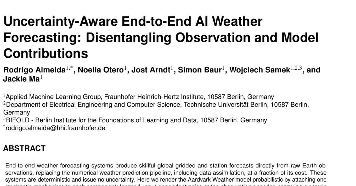
End-to-end weather forecasting systems produce skillful global gridded and station forecasts directly from raw Earth observations, replacing the numerical weather prediction pipeline, including data assimilation, at a fraction of its cost. These systems are deterministic and issue no uncertainty. Here we render the Aardvark Weather model probabilistic by attaching one stochastic mechanism to each component: learned, input-dependent noise at the observation encoder, capturing aleatoric uncertainty inherited from the observing system, and Monte Carlo dropout in the processor, capturing epistemic uncertainty in the learned dynamics. The resulting nested ensemble attributes forecast spread to the two sources through a law-of-total-variance decomposition, cross-checked by withholding observation streams. Probabilistic finetuning significantly improves the mean forecast, by 4.2% on average across variables and lead times. The ensemble is calibrated against ERA5 through the medium range (spread-skill ratio 0.98), keeps station RMSE within 2.4% of the deterministic model while beating it in CRPS at every lead time, and trails the operational ECMWF ensemble. The encoder branch behaves as observation-driven uncertainty. Component-attributed uncertainty makes end-to-end forecasts more transparent, a step toward observation-driven digital twins of the atmosphere.