Latent-IMH: Efficient Bayesian Inference for Inverse Problems with Approximate Operators

AI summary

Overview

Research area: Bayesian inference and Markov chain Monte Carlo (MCMC) for high-dimensional linear inverse problems, spanning computational statistics, numerical linear algebra, and scientific computing.

Technical level: Advanced. The paper combines linear operator factorization (SVD reparameterization, Helmholtz and graph Laplacian operators) with Bayesian non-asymptotics (KL divergence closed forms, total-variation mixing time bounds).

Scope: The paper introduces Latent-IMH, an independence Metropolis-Hastings sampler that uses a cheap approximate operator to build proposals for a latent variable and the expensive exact operator to refine them, and analyzes it both theoretically and empirically against Approx-IMH, NUTS, MALA, and two-stage multi-fidelity MCMC.

What This Paper Is About

Many Bayesian inverse problems assume observations of the form y = A x, where applying A is computationally expensive because it involves inverting a large physics operator (for example a discretized PDE). Sampling the posterior p(x|y) therefore costs a large number of expensive linear solves. This paper asks whether an inexpensive approximation à of A can be used to do most of the sampling work while still targeting the exact posterior, and how much that helps.

Key Contributions

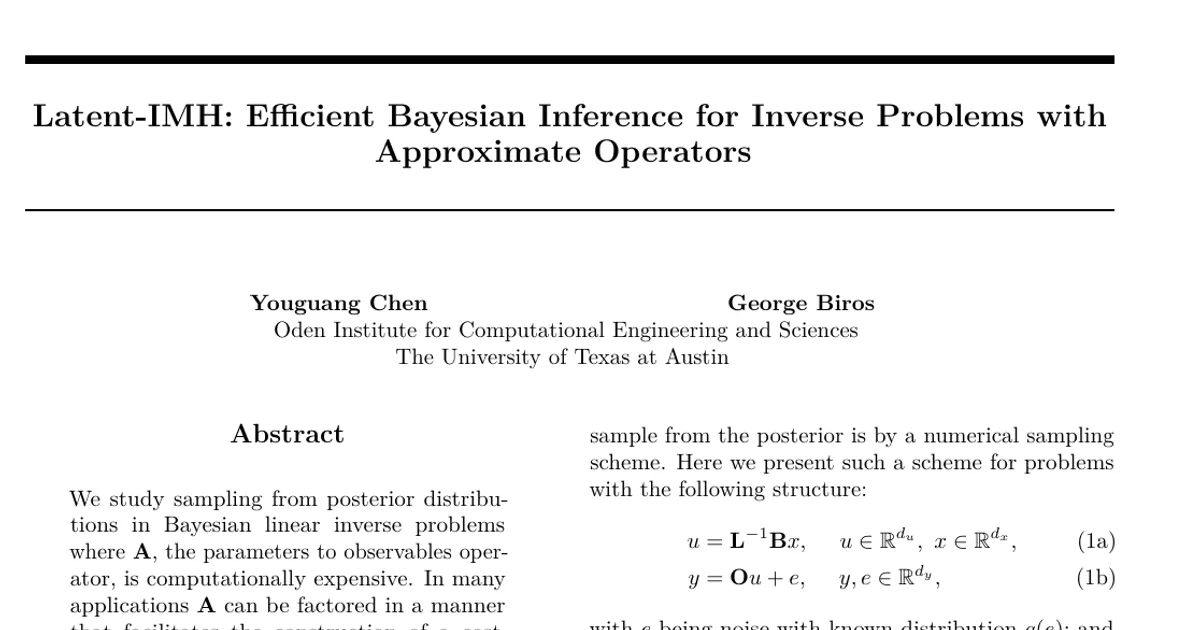
1. A latent-variable proposal distribution. Latent-IMH first draws a latent variable u from an approximate posterior π_a(u|y) ∝ q(y − Ou) p̃(u) built with the cheap operator, then maps it back to the parameter space via x ← F⁻¹u, where F = L⁻¹B. The corresponding posterior is π_l(x|y) ∝ q(y − Ax) p̃(Fx).

2. A theoretical comparison of Approx-IMH and Latent-IMH via KL divergence. Under Gaussian prior and Gaussian noise assumptions, the paper derives closed-form expressions for the expected KL divergence (Proposition 3.2), an exact diagonal-case expression (Proposition 3.3), and general upper bounds (Theorem B.2).

3. New mixing time bounds. Theorem 4.3 establishes general mixing time bounds for both samplers under strong log-concavity and local Lipschitz assumptions on the log-weight functions, and Theorem 4.4 gives the scaling in a diagonal case, showing Approx-IMH scales as 𝒪(d² d_y² ‖A‖⁴/σ⁴) while Latent-IMH scales as 𝒪(d²).

4. Numerical experiments comparing Latent-IMH against Approx-IMH, NUTS, MALA, and two-stage (delayed-acceptance) MCMC on Gaussian, ill-conditioned Gaussian, Gaussian mixture, Laplace-with-normalizing-flow, graph Laplacian, and acoustic scattering problems.

Main Findings

• Latent-IMH reaches a target accuracy with far fewer exact solves. For 10% relative mean error on the acoustic source reconstruction, Latent-IMH requires ∼10³ solves, Approx-IMH ∼10⁵, and MALA/NUTS millions of solves.

• The acceptance ratio of Latent-IMH does not contain the likelihood term. In Eq. 8, the noise distribution q() vanishes from the acceptance ratio, which the authors state makes it quite accurate when the noise is small.

• Latent-IMH is more robust to noise level and observation ratio than Approx-IMH. Both expected KL divergences D_a and D_l increase with spectral error and problem dimension, but D_a is highly sensitive to noise level and the observation ratio d_y/d, while D_l is not. The final term of D_l scales as 𝒪(δσ²/s_i²), compared with 𝒪(δ²s_i²/σ²) for D_a, where δ = |α_i − 1|.

• Approx-IMH degrades in low-noise or high-observation regimes. Because its mixing time scales with ‖A‖⁴/σ⁴ and d_y², Approx-IMH can mix much more slowly when noise is low or the proportion of observations is high.

• Latent-IMH wins on multimodal and non-Gaussian priors. With a three-component Gaussian mixture prior, Latent-IMH consistently outperforms the other methods, and local MCMC methods such as NUTS exhibit poor mixing in multimodal settings due to barriers between modes.

• With a Laplace prior and a normalizing flow, Latent-IMH outperforms both Approx-IMH and NUTS; Latent-IMH and NUTS achieve similar convergence rates, while Approx-IMH frequently rejects proposals and stagnates.

• On the graph Laplacian problem with PCG approximation (d_u = 8,000, d_x = 800, d_y = 160), Latent-IMH at a PCG tolerance of 0.1 outperforms Approx-IMH at a much stricter tolerance of 5×10⁻⁴, even though Approx-IMH has a higher acceptance rate of 34.2%.

• Acceptance ratio sensitivity tests show that as spectral error or dimensionality increases, acceptance ratios decline for both methods, but much more sharply for Approx-IMH.

Methodology in Plain English

The authors exploit a structural decomposition of the forward model. The observation y is written as y = OFx, where B lifts the unknown parameters into the input space of a physics operator L, and F = L⁻¹B. Because L is expensive to invert, they assume an approximation L̃ satisfying L̃⁻¹L ≈ I (for example incomplete factorizations, approximate graph Laplacians, truncated Krylov solvers, multigrid solvers, or approximate hierarchical matrices), with L̃⁻¹ potentially 10× or more faster than L⁻¹.

Two samplers are built on this. Approx-IMH simply replaces A with à = OF̃ everywhere, proposing directly in x-space. Latent-IMH instead proposes in a latent u-space using the cheap operator, then maps proposals to x with the exact inverse F⁻¹. Both are used as independence proposals g(x|y) inside the standard IMH algorithm, so the acceptance ratio corrects for the mismatch between the proposal and the exact posterior — which is why the exact operator is still needed, but only once per step.

To make the latent construction well-posed, the authors assume d_x ≤ d_u and d_y ≤ d_x, use an SVD of the observation operator O to build a reparameterization matrix V_x and a modified observation operator Z = OV_x, and reduce to the square case where F is invertible. The latent prior p̃(u) can be set as the pushforward p(F̃⁻¹u)|det F̃⁻¹| or learned with a normalizing flow or variational autoencoder. The theoretical work then compares the two posteriors' KL divergence from the exact posterior and their mixing times under log-concavity assumptions.

Why This Matters

Impact on research. The paper reframes the use of approximate operators in MCMC: instead of using them for local, state-dependent screening (as in delayed-acceptance methods) or for coupled variance reduction (as in multilevel MCMC), it uses them to construct independent proposals that can be precomputed and evaluated in parallel. Its analytic KL and mixing time bounds give a concrete criterion for when this pays off.

Real-world applications (drawn from the paper's list of inverse problems admitting the y = OFx formulation):

• Electrical impedance tomography.
• Acoustic and electromagnetic scattering, including the time-harmonic Helmholtz problem where L = k²I + Δ.
• Exploration geophysics and photoacoustic and optical tomography.
• Graph inference tasks, such as reconstructing unknown node values or edge weights from partially known vertex features, and image processing.

Industry relevance. Any pipeline that repeatedly solves a large linear system inside a Bayesian sampling loop — medical and seismic imaging, acoustic source localization, sensor-network and graph-based estimation — can potentially shift most of its compute into an offline phase and reserve the exact operator for a single refinement per sample. The reported gap (∼10³ solves versus millions) is directly a compute-budget and latency argument.

Future Directions

• Broader theory beyond log-concavity. Assumption 4.1 requires the exact posterior to be strongly log-concave, and the mixing time analysis assumes locally Lipschitz log-weight functions; extending the guarantees to weakly log-concave or multimodal posteriors remains open.

• Better learned latent priors. The paper allows p̃(u) to be built with normalizing flows or variational autoencoders, and demonstrates a normalizing flow in the Laplace-prior experiment; how to train these priors reliably and how their error interacts with the operator approximation error is not fully resolved.

• Nonlinear and non-Gaussian observation models. The formulation and all analysis assume a linear observation operator O and a fixed noise distribution, and the acoustic scattering experiment (the last one presented) is described only up to its operator construction in the supplied text.

• Choosing the approximate operator and its tolerance systematically. The graph Laplacian experiment shows that Latent-IMH at a loose PCG tolerance can beat Approx-IMH at a strict one, suggesting a cost-accuracy trade-off curve that is not yet characterized analytically.

Target Audience

Researchers and practitioners in computational statistics, uncertainty quantification, and scientific computing who work on Bayesian inversion with expensive forward models. It is most useful to readers already comfortable with MCMC accept/reject mechanics, Gaussian posterior algebra, KL divergence, and the numerical linear algebra of preconditioners and factorizations. Readers looking for a plug-in sampling method rather than theory will find the algorithmic template in Section 2 and the acceptance ratios in Eq. 7 and Eq. 8 most immediately actionable.

Authors’ abstract

We study sampling from posterior distributions in Bayesian linear inverse problems where $A$, the parameters to observables operator, is computationally expensive. In many applications, $A$ can be factored in a manner that facilitates the construction of a cost-effective approximation $\tilde{A}$. In this framework, we introduce Latent-IMH, a sampling method based on the Metropolis-Hastings independence (IMH) sampler. Latent-IMH first generates intermediate latent variables using the approximate $\tilde{A}$, and then refines them using the exact $A$. Its primary benefit is that it shifts the computational cost to an offline phase. We theoretically analyze the performance of Latent-IMH using KL divergence and mixing time bounds. Using numerical experiments on several model problems, we show that, under reasonable assumptions, it outperforms state-of-the-art methods such as the No-U-Turn sampler (NUTS) in computational efficiency. In some cases, Latent-IMH can be orders of magnitude faster than existing schemes.