Gradient Variance Reveals Failure Modes in Flow-Based Generative Models

AI summary

Overview

Research area: Generative modeling — specifically flow matching, Rectified Flows (ReFlow), optimal transport (OT), and memorization versus generalization in diffusion- and flow-based samplers.

Technical level: Advanced. The paper mixes closed-form optimal-transport derivations, gradient-variance analysis, and propositions proved under Lipschitz/linear-growth assumptions, alongside empirical work on synthetic Gaussians and CelebA.

Scope in one sentence: The paper uses the variance of the training-loss gradient to explain which vector fields optimization favors in flow-based generative models, and shows that deterministic (noiseless) interpolants drive memorization of arbitrary training pairings while a small amount of injected noise restores generalization.

What This Paper Is About

Rectified Flows learn ODE vector fields whose trajectories are supposed to be straight between a source distribution and a target distribution, which would allow near one-step sampling. The authors argue that this straight-path objective hides fundamental failure modes: under deterministic training, low gradient variance pushes the model to memorize whatever source–target pairings it was trained on, even when the straight interpolant lines between those pairs intersect. The goal is to characterize, theoretically and empirically, which vector fields optimization favors in stochastic versus deterministic regimes, and to show that the resulting memorization is reproduced exactly at inference time.

Key Contributions

1. A gradient-variance analysis in the Gaussian-to-Gaussian setting (Section 3). The authors ask "when is gradient variance informative?" and show the answer depends on the training regime. They derive closed-form expressions for the optimal vector field, derive bounds for the loss and gradient variance under both regimes, and show empirically that observations align with the predictions of Proposition 1. Figure 6 is presented as the central illustration.

2. An extension from Gaussians to general finite datasets within the ReFlow paradigm (Section 4). Proposition 2 proves that a vector field minimizing the loss exists that corresponds exactly to the pairings seen in the data, and Remark 1 explains that because integration is deterministic, the model can reproduce these exact pairings at inference by effectively "jumping over" intersections.

3. Two supporting theoretical results. Lemma 2 establishes the idempotence of Rectified Flows (subsequent ReFlow iterations with a noise-free interpolant yield identical couplings), and Counter-Example 1 shows that 1-Reflow is not sufficient to guarantee straight paths under mild assumptions.

4. Empirical validation on a Mixture of Gaussians and CelebA. Section 4.2 tests memorization on a Gaussian mixture in low ($d=3$) and high ($d=50$) dimensions, and Section 4.3 tests it on CelebA using optimal-transport pairings from Korotin et al. (2021) as reference.

Main Findings

• Gradient variance is not driven by geometric proximity of interpolants. A common misconception in flow matching is that gradient variance originates where straight-line interpolants intersect. Proposition 1 challenges this: variance can be nonzero even for straight couplings with no intersections, while intersections or regions of high interpolant density do not by themselves induce elevated variance. In Figure 5, with a $180^\circ$ rotation all interpolants intersect at $t=1/2$, yet variance is lowest there.

• Variance is governed by mismatch between the learned vector field and the pairing structure. Under the optimal transport (OT) field, random pairings exhibit lower variance than structured pairings with $120^\circ$ (straight) or $180^\circ$ (not straight) rotations. With a non-OT vector field, the loss can display substantial variance for pairings that are themselves OT.

• Low gradient variance does not certify transport optimality. For the OT field and the rotational OT (rOT) field, Proposition 1 shows zero loss and zero gradient variance when the field and the pairings are aligned. When they are aligned (e.g., both apply the same rotation) both loss and gradients vanish, whereas under the OT field even straight pairings can exhibit nonzero gradient variance.

• Memorization in the intersecting-pairing experiment. With $X_0 \sim \mathcal{N}(0, I_2)$ and $X_1 = R_{180^\circ}X_0 + [5,5]^\top$, all straight-line interpolants meet at the midpoint $t = 1/2$. Under noiseless interpolants the learned vector field memorizes this ill-defined pairing and, at inference, reproduces the same mapping that rotates the source Gaussian by $180^\circ$ and translates it by $[5,5]^\top$. The stated reason: the probability of sampling exactly $t = 1/2$ during training is zero, so the field is never constrained at the intersection, and deterministic numerical integration bypasses the singular location.

• Noise shifts preference toward the optimal field. In Figure 4, for the pairing $(X_0, R_{30^\circ}X_0 + \mu)$, as the noise level increases ($\sigma = 0 \to 4$) the OT field exhibits significantly reduced variance ($p < 0.01$, paired t-test) while maintaining lower transport error. With noisy interpolants, the optimal vector field exhibits lower gradient variance than the pairing-optimal field, and at $t=1/2$ the gradient variance becomes very high even though that time point is never sampled.

• Rectified Flow stagnates on straight couplings. Lemma 2 states that for a straight-line coupling via the linear interpolant, $\texttt{ReFlow}^{(k)}(Z_0, Z_1) = (Z_0, Z_1)$ for all $k \geq 1$. The paper notes this was previously established in Roy et al. (2024) and Liu (2022).

• 1-Reflow can fail. Counter-Example 1: even if the learned transport map $T(x_0)$ is injective (e.g., under standard Lipschitz and growth conditions), the straight-line interpolant need not be. A rotation-based map such as $T(x_0) = R_{180^\circ}x_0 + 5$ produces overlapping interpolants, breaking injectivity of $(x_t, t) \mapsto x_0$.

• The minimizer memorizes (Prop. 2). For a finite dataset of $N$ i.i.d. samples ${Z_0^{(i)}, Z_1^{(i)} = T(Z_0^{(i)})}$ with $m$ sampled time points each, there exists a deterministic vector field attaining zero loss on the empirical objective. Remark 1 adds that to actually recover the original pairings, integration must traverse the specific sampled time steps — the only points where $v(x_t,t) = x_1 - x_0$ is guaranteed.

• Noise breaks the proof assumptions. Noisy interpolants break the bijection between $(x_t, t)$ and $(x_0, T(x_0))$, violating key steps in the proofs of Lemma 2 and Proposition 2, and preventing the model from getting stuck in deterministic straight pairings.

• Why CFM does not memorize random pairings. In standard Conditional Flow Matching, $x_0$ is sampled independently from a continuous distribution each epoch. The authors initially hypothesized CFM could memorize random couplings, but the independent sampling breaks the bijection between $(x_t, t)$ and $(x_0, x_1)$ — the same mechanism as Remark 2.

• Gaussian mixture results (Table 1). Comparing CFM and CFM($\sigma=0.05$) at $d=3$ and $d=50$ on log-likelihood under the true mixture, MMD, and Sinkhorn distance, with four comparisons (Gen, Mem, True, Data) and results averaged over 10 seeds. CFM tends to memorize the deterministic pairings it is trained on — reflected in very low memorization MMD values ($1.758\times10^{-06}$ at $d=3$ and $9.089\times10^{-06}$ at $d=50$) — but shows weaker generalization (Gen MMD $0.0034$ at $d=3$ and $0.0021$ at $d=50$). CFM($\sigma=0.05$) shows lower distances to the true distribution (Gen MMD $0.0018$ at $d=3$ and $0.0020$ at $d=50$; Gen Sinkhorn $0.0680$ at $d=3$ versus $0.0730$, and $15.1689$ at $d=50$ versus $15.1900$), indicating superior generalization and less reliance on memorized pairings.

• CelebA adversarial pairings (Table 2). Targets of the Korotin et al. (2021) optimal OT pairings were shuffled to produce random pairings with no coherent OT semantics, evaluated on held-out subsets of 5K and 50K samples. CFM($\sigma=0$) strongly memorizes the shuffled targets: 5K memorization (L2 to shuffled) $28.57 \pm 5.49$ versus CFM($\sigma=0.05$) $55.02 \pm 16.51$; 50K memorization $45.98 \pm 11.85$ versus $56.48 \pm 18.55$. Conversely, CFM($\sigma=0.05$) generalizes better: 5K generalization (L2 to OT) $34.25 \pm 7.54$ versus $50.40 \pm 16.73$, and 50K generalization $30.05 \pm 6.77$ versus $46.78 \pm 14.87$.

• Simulated 1-ReFlow (Table 3). A base CFM model is trained on random (non-OT) pairings, used to generate endpoints by ODE integration, and CFM is then retrained on those generated endpoints. The pattern is consistent: CFM($\sigma=0$) shows stronger memorization (5K memorization L2 to generated $8.63 \pm 1.76$ versus $25.08 \pm 8.59$ for CFM($\sigma=0.05$)), while CFM($\sigma=0.05$) generalizes better (5K generalization $31.35 \pm 7.38$ versus $43.35 \pm 14.21$; 50K generalization $32.54 \pm 8.86$ versus $38.16 \pm 11.37$).

• Dataset size matters. Memorization effects diminish with larger datasets, since fixed model capacity makes perfect memorization infeasible for 50K samples compared with 5K. Optimization still favors memorization when possible, as predicted by Proposition 2.

• A negative representational result. Lemma 1 shows that the closed-form OT vector field $v_{OT}$ cannot be exactly represented by an MLP, CNN, or Transformer architecture given concatenated inputs $[X_t, t]$; the paper attributes this to the difficulty of capturing the matrix inverse term $[I + t\Theta]^{-1}$.

Methodology in Plain English

The authors deliberately start with a case they can solve by hand: transporting one Gaussian distribution to another. In that setting the optimal vector field has a known closed form, so instead of approximating it with a neural network they plug in the exact formula and compute the loss and the variance of its gradients analytically across many configurations — different pairing schemes (optimal transport, rotated, random), different interpolants (noiseless versus noisy), and different vector-field classes including a "rotating OT" field that first rotates the source and then maps it to the target.

They then measure the same quantities numerically using Monte Carlo estimates over finite sample batches, using 100 bootstrap samples for 95% confidence intervals, and check whether the empirical numbers match the theoretical ones. A key design choice is a pairing where every straight interpolant line crosses the same point at $t=1/2$, which lets them test whether intersections are what cause gradient variance.

In the second half they move from Gaussians to general finite datasets. They prove two statements: that Rectified Flow stops changing once it reaches a straight coupling, and that a vector field achieving zero empirical loss exists that exactly encodes the training pairs. They then test

Authors’ abstract

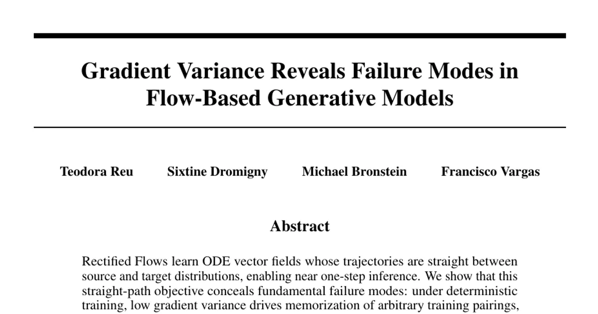
Rectified Flows learn ODE vector fields whose trajectories are straight between source and target distributions, enabling near one-step inference. We show that this straight-path objective conceals fundamental failure modes: under deterministic training, low gradient variance drives memorization of arbitrary training pairings, even when interpolant lines between pairs intersect. To analyze this mechanism, we study Gaussian-to-Gaussian transport and use the loss gradient variance across stochastic and deterministic regimes to characterize which vector fields optimization favors in each setting. We then show that, in a setting where all interpolating lines intersect, applying Rectified Flow yields the same specific pairings at inference as during training. More generally, we prove that a memorizing vector field exists even when training interpolants intersect, and that optimizing the straight-path objective converges to this ill-defined field. At inference, deterministic integration reproduces the exact training pairings. We validate our findings empirically on the CelebA dataset, confirming that deterministic interpolants induce memorization, while the injection of small noise restores generalization.