Convex Dominance in Deep Learning I: A Scaling Law of Loss and Learning Rate

AI summary

Overview

• Research area: Optimization theory and empirical scaling laws for deep learning (training dynamics, learning rate schedules, loss prediction).
• Technical level: Advanced. The paper builds on convex optimization convergence proofs (SGD upper bounds, Lipschitz/bounded-gradient conditions) and requires familiarity with learning rate schedules, optimizer variants (AdamW, Muon, SGD, LoRA), and scaling-law conventions.
• Scope: One-sentence scope: the paper argues that deep learning loss landscapes behave as if weakly convex after a short warm-up, and uses that assumption to derive a single scaling law that simultaneously predicts loss and the optimal peak learning rate across training horizons and model sizes.

What This Paper Is About

Deep learning loss landscapes are non-convex, with many local minima and saddle points, so optimization behavior is normally hard to analyze or control. This paper asks whether the loss dynamics of real deep learning training can be treated as convex-like — specifically, weakly convex with bounded gradients — and whether that treatment is precise enough to predict loss from the learning rate schedule. The goal is a scaling law that predicts both the loss and the optimal peak learning rate, and that extrapolates across training horizons and model sizes.

Key Contributions

1. A general mapping from learning rate sequence to loss sequence. The authors study convex-like behavior in deep learning across general model architectures, optimizers, and learning rate schedules, establishing a non-asymptotic mapping from the learning rate sequence to the loss sequence.
2. An asymptotic loss upper bound with O(1/√T) convergence. They generalize to an asymptotic bound achieving O(1/√T) convergence under two conditions: (I) the peak learning rate is scaled by 1/√T, and (II) the learning rate schedule is "qualified."
3. A qualification exam for schedules. They give a training-free, symbolic test (Condition 2.5) that determines whether a schedule can achieve the optimal O(1/√T) rate, without running any model optimization.
4. A data-driven scaling law. They propose fitting the asymptotic bound empirically, yielding a scaling law across training horizons and model sizes that predicts loss and optimal learning rate together.

Main Findings

• Constant learning rate is suboptimal. Under the convex analysis, a constant schedule achieves only O(√(ln T / T)), with optimal bound L* + DG√(ln T / T) and optimal peak learning rate η_peak*(T) = D / (G√(ln T · T)).
• Square-root inverse also fails the exam. The η_peak/√t schedule achieves L* + DG√(ln T / (4T)), better than constant but still not O(1/√T).
• Linear, cosine, and warmup-stable-decay (WSD) schedules are "qualified." Linear decay gives L* + 2DG√(1/T) with η_peak*(T) = D/(G√T); cosine decay gives L* + 2DG√(1.061/T) with η_peak*(T) = D/(G√(1.061T)). WSD depends on a parameter c through the term 1 + ½ ln((1+c)/(1−c)).
• Qualified schedules share two traits: they are horizon-aware (η_t depends on T), and their loss bounds take the form L_SGD-last(η_peak, T) = L* + q₁²/(Tη_peak) + η_peak q₂² for constants q₁, q₂.
• Any rescaled peak learning rate still converges optimally. Corollary 2.4 shows that for any η_ref > 0 with η_peak = η_ref/√T, the excess loss behaves as Q(η_ref)/√T where Q(η_ref) = q₁²/η_ref + η_ref q₂²; the optimum is η_ref* = q₁/q₂ and the resulting excess loss is 2q₁q₂/√T.
• Convex-like bounds hold empirically in deep learning. A generalized bound (Generalization 1) fits ResNet18 on ImageNet with SGD and with AdamW, and GPT2 (124M) on OpenWebText with AdamW and Muon-NSGD, with R² scores ≥ 0.95 when half the iterations are used to fit and half to predict.
• Fit holds for dense and MoE language models. Using losses from Li et al. (2025) for dense and Mixture-of-Experts models trained with AdamW and cosine decay, R² across model sizes and architectures is ≥ 0.95.
• Chinchilla-style data confirms the last-iterate law. On models from 0.074B to 12.56B in Hoffmann et al. (2022), reconstructed by Besiroglu et al. (2024), the fit gives R² ≥ 0.978, up to FLOPs = 1e22 and over 300B tokens; all loss values are within 1% relative error of prediction. As model size grows, L̃_∞ decreases log-linearly and 2q̃₁q̃₂ roughly increases.
• Extrapolation magnitude. The scaling law extrapolates about 80× across training horizons and about 70× across model sizes. Optimal η_ref* was 10 for Muon-NSGD and 0.3 for AdamW in the GPT2 (0.1B) experiments.
• Predictive very early. Good linear fits over 1/√T < 0.02, i.e. T > 2.5k iterations, for GPT2 (0.1B) trained from 100 to 500k steps.
• Generalizes to multi-modal models. A VLM of about 1B parameters fine-tuned on Cauldron with AdamW and cosine decay (3% warmup) fits well when T > 2000, with all component learning rates (language backbone, vision backbone, modality projector) 1/√T-scaled.
• Known limitation. The approach fails to predict test loss and continues to predict training loss when overfitting is severe (Figure 12); the paper also does not explain why convex-like behavior arises across architectures or how many iterations it takes to emerge.

Methodology in Plain English

The authors start from textbook convex optimization. Under a convexity condition and a bounded-gradient condition (E‖g(w)‖² ≤ G²), the SGD update rule yields a closed-form upper bound on the loss at any iterate — the bound depends on the learning rate sequence, the distance D from initialization to the optimum, and the gradient bound G. Plugging in specific schedules (constant, square-root inverse, linear decay, cosine decay, WSD) produces per-schedule formulas for the loss bound, and minimizing each over the peak learning rate yields the optimal schedule-specific learning rate (Table 1).

A key step: because deep learning does not satisfy convexity literally, the authors relax the bound. They replace the exact constants with fitted ones (D̃, G̃, L̃_∞ instead of D, G, L*), rename the irreducible floor as the loss at the limit of training rather than a unique global minimum, and refit the resulting expression to observed loss curves by non-negative linear regression. Half the iterations of a run are used to fit; the other half are used to test the prediction. They repeat this for several optimizers (SGD, AdamW, Muon-NSGD, LoRA), architectures (ResNet, ViT, GPT2, a vision-language model with LLAMA3 backbone), datasets (ImageNet, OpenWebText, Cauldron), and schedules.

For the scaling law, they run 240 GPT2 training runs on OpenWebText spanning 4 settings (0.1B/AdamW, 0.1B/Muon-NSGD, 1B/Muon-NSGD, 7B/Muon-NSGD), 10 training horizons from 100 to 500k iterations, and 6 values of η_ref from 0.01 to 30.0. The fitted line over 1/√T gives the intercept (L̃_∞) and slope (Q̃), and the optimal η_ref is read off the linear fit. They then transfer the η_ref from the small model to larger models using η_peak*(N,T) ≈ η_peak*(N_small, T_small)/√(T/T_small).

Why This Matters

• Impact on research: It extends one-line-of-work findings (notably Schaipp et al. 2025, which also builds on Defazio et al. 2023) by covering arbitrary schedules theoretically and by validating across models, optimizers, and horizons. It contrasts with prior learning rate scaling laws that report exponents such as α = 0.125 (Bi et al. 2024) or α ∈ {0.32, 0.38, 0.42, 0.65, 0.70} (Bjorck et al. 2024, Table 5) or horizon-unaware laws with α = 0, because this paper predicts loss and learning rate jointly at a fixed α = 0.5.
• Challenges a common assumption: It argues that claims of learning-rate transfer across training horizons from maximal update parameterization (muP, Yang et al. 2022) contradict empirical evidence in Bjorck et al. (2024) and this paper's analysis.
• Real-world applications:
  • Choosing the peak learning rate for a long training run from short, cheap pilot runs.
  • Designing schedules that qualify for O(1/√T) convergence rather than suboptimal O(√(ln T / T)).
  • Predicting final loss curves for compute budgeting before committing to full-scale training.
  • Transferring hyperparameters from a small model to a larger one (0.1B to 1B to 7B in this paper).
• Industry relevance: The method is data-driven and cheap — the qualification exam is training-free and the scaling law is fit from small-scale runs, with reported extrapolation of about 80× in horizon and 70× in model size, plus validation on Chinchilla-scale runs up to 12.56B parameters and FLOPs = 1e22.

Future Directions

1. Explain why convex-like behavior emerges. The paper explicitly notes it lacks understanding of why this behavior appears across architectures.
2. Characterize the warm-up length. It is unresolved how many iterations are needed before deep learning becomes characterizable by convex-like bounds.
3. Fix the overfitting failure case. The method predicts test loss poorly and keeps predicting training loss when overfitting is severe; extending it to test loss or generalization is an open problem.
4. Broaden the empirical base further. The authors already test LoRA and run ablations over weight decay, gradient clipping, momentum coefficient, batch size, and random seeds, but richer optimizer and architecture coverage remains a natural next step.

Target Audience

This paper is best suited for machine learning researchers and engineers who work on large-scale training: practitioners tuning learning rate schedules, researchers studying scaling laws, and optimization theorists interested in how far convex analysis transfers to non-convex deep learning. It assumes comfort with convergence rates, SGD proofs, and optimizer terminology, so it is not aimed at beginners, though the takeaway formulas (optimal peak learning rate scaling as 1/√T and loss decaying as O(1/√T)) are usable by anyone who trains models at scale.

Authors’ abstract

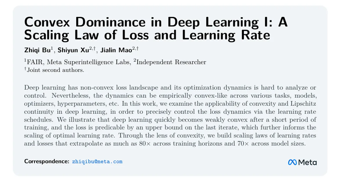
Deep learning has non-convex loss landscape and its optimization dynamics is hard to analyze or control. Nevertheless, the dynamics can be empirically convex-like across various tasks, models, optimizers, hyperparameters, etc. In this work, we examine the applicability of convexity and Lipschitz continuity in deep learning, in order to precisely control the loss dynamics via the learning rate schedules. We illustrate that deep learning quickly becomes weakly convex after a short period of training, and the loss is predicable by an upper bound on the last iterate, which further informs the scaling of optimal learning rate. Through the lens of convexity, we build scaling laws of learning rates and losses that extrapolate as much as 80X across training horizons and 70X across model sizes.