Back to the Future: Look-ahead Augmentation and Parallel Self-Refinement for Time Series Forecasting

AI summary

Overview

• Research area: Long-term time series forecasting (LTSF), specifically data augmentation and ensembling for linear forecasting models. Published at the ACM Web Conference 2026 (WWW '26).
• Technical level: Intermediate. The method itself is conceptually simple, but understanding it benefits from familiarity with standard forecasting terminology (direct vs. iterative multi-step forecasting, horizon, MSE/MAE, ensembling).
• Scope: The paper proposes BTTF ("Back to the Future"), a two-stage training framework that feeds a model's own initial forecasts back in as augmented input to refine long-horizon predictions in parallel.

What This Paper Is About

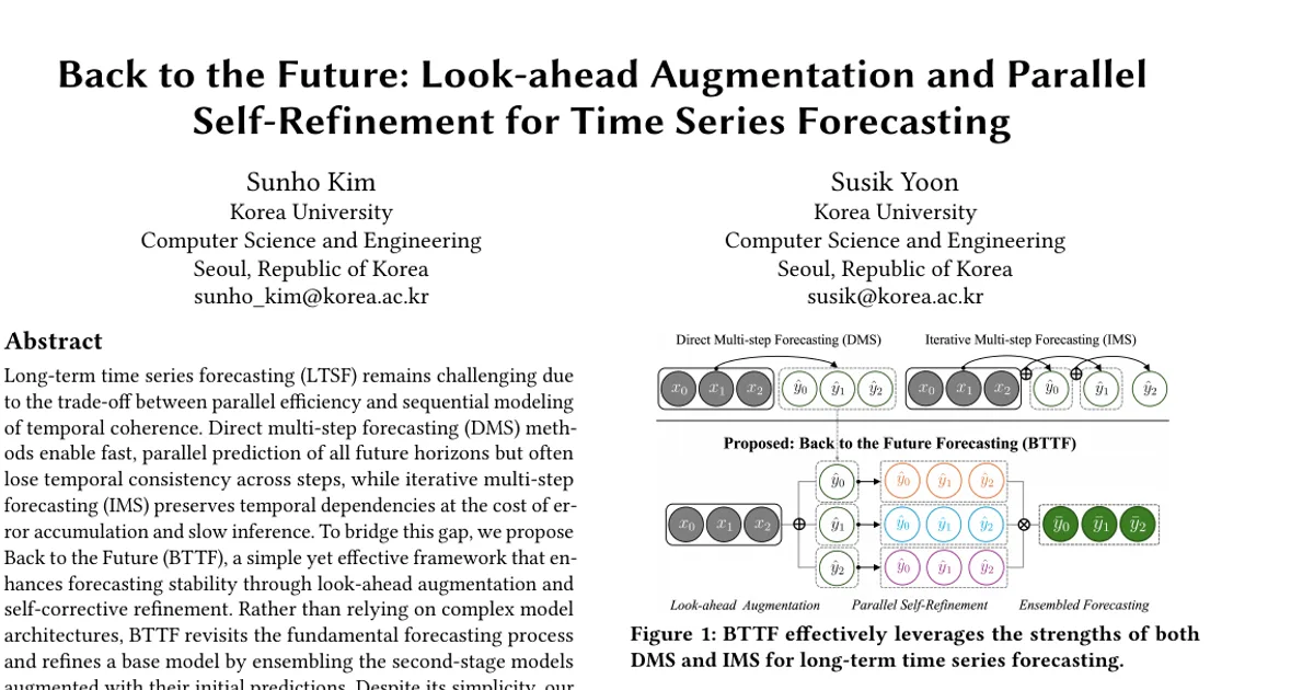
Long-term forecasting faces a trade-off: direct multi-step (DMS) models predict all future steps at once (fast, parallel, but weak temporal consistency), while iterative multi-step (IMS) models predict step by step (temporally coherent, but slow and prone to error accumulation). The paper asks whether a simple linear model can get the benefits of both by treating its own first-pass forecast as an extra input feature rather than as the final answer. Instead of designing a more complex architecture, the authors augment the input with segments of the initial prediction and train multiple second-stage models to refine it.

Key Contributions

1. The authors state this is the first work to simultaneously combine an IMS-like use of future predictions with DMS-like parallelism for LTSF.
2. They instantiate the idea on simple linear models (Linear and DLinear) through a systematic two-stage training scheme: look-ahead augmentation plus parallel self-refinement.
3. They add a step-wise top-K ensembling procedure that ranks second-stage models by validation performance and chooses the ensemble size K* using observable prediction statistics (variance and mean correlation) as surrogates for the bias–variance–covariance decomposition of ensemble error.
4. Experiments show up to 58% performance improvement for linear models on the benchmark datasets, including cases where first-stage training was unstable.

Main Findings

• Consistent gains on most settings: Applying BTTF to Linear and DLinear improves accuracy in most configurations and often reaches competitive or superior performance versus iTransformer and SegRNN.
• Largest gains on ILI: For Linear+BTTF (1E-1E) at horizon 24 on ILI, MSE drops from 1.6197 to 0.6682 (58.7% improvement) and MAE from 1.1315 to 0.6547 (42.1%). The abstract and conclusion describe this as "up to 58%."
• Robust to a weak first stage: Even when the first-stage model is poorly optimized due to unstable or insufficient training, the second-stage models often beat the best reported base-model performance, with improvements of up to 35% (seen on Exchange Rate, horizon 192, DLinear+BTTF 1E-1E: MSE 0.3080 to 0.2001).
• The cheapest setting works: The simplest 1E–1E configuration (one epoch for both stages) still yields strong results, suggesting the step-wise ensemble efficiently exploits diverse models.
• ETTm2 is the exception: Where the first-stage model is already sufficiently fitted, BTTF produces a slight drop of around 2% on average. The authors frame this as BTTF doubling as a diagnostic for whether a base model has room for improvement.
• Occasional regressions elsewhere: On Linear at ETTh1 horizon 720, the 1E-1E setting degrades MSE by 4.1% and MAE by 2.0%; on Exchange Rate horizon 192, Linear+BTTF (ES-1E) shows a 0.4% MAE regression.
• Modest overhead: The first-stage training time is unchanged (it is identical to the base model). The second stage adds roughly 8.3x training time on average, but overall processing time averages 2.6x that of iTransformer and SegRNN, and is 21% lower than those baselines on the ILI dataset. The second-stage models are independent and can be distributed across processing units.

Methodology in Plain English

The framework has three stages.

1. Look-ahead augmentation. First, a base model is trained normally and produces an H-step forecast. That forecast is cut into N fixed-length segments (the segmentation window is set to one-third of the prediction horizon). Each segment is appended to the original historical input window, producing N augmented inputs that share the same history but carry a different slice of the first-stage forecast.

2. Parallel self-refinement. One second-stage model is trained per augmented input, all predicting the same H-step horizon. Because each model sees a different piece of the initial forecast, each learns a different correction direction — effectively an implicit residual adjustment even though no explicit residual model is used. All of these models can be trained in parallel.

3. Ensembled forecasting. Second-stage models are ranked by validation performance. Predictions from the top-K models are averaged, with K swept from M up to N in increments of M (the step size is fixed to M = 5). To pick K*, the authors use observable prediction statistics — variance V(K) and mean correlation R(K) — as practical stand-ins for the variance and covariance terms in the standard ensemble error decomposition (Ueda and Nakano, 1996), combined in a min–max normalized score S(K). The K minimizing S(K) is chosen. High variance flags outlier predictors; high correlation flags redundant ones.

Experimental setup: Four benchmarks (ETTh1, ETTm2, Exchange Rate, ILI) in the univariate forecasting setting. Base models are Linear and DLinear from the official LTSF-Linear implementation; comparisons use iTransformer and SegRNN from the Time-Series-Library benchmark. Accuracy is measured with MSE and MAE across multiple horizons. The segmentation stride is 1 for ILI and {1, 2, 4, 8} for the other datasets. Base and second-stage models use identical hyperparameters.

Why This Matters

The paper argues that progress in LTSF has been dominated by architectural complexity, and that a lightweight linear model combined with augmentation and self-refinement can outperform or match far heavier designs. It reframes forecasts as reusable features rather than final outputs, bridging architecture-centric (DMS-style) and data-centric (IMS-style) paradigms.

Real-world applications implied by the paper's stated domains:

• Finance / Exchange Rate forecasting — currency series, where the exchange rate benchmark is used directly.
• Transportation — cited as a core time series forecasting domain.
• Web-scale services — cited as a domain where LTSF supports reliability and adaptive decision-making as internet systems scale.
• Energy and public health — the ETTh1/ETTm2 electricity transformer temperature datasets and the ILI influenza-like illness dataset are the evaluation targets.

Industry relevance: The approach adds a second training stage to an existing model rather than requiring a new architecture, and the second-stage models are independent and parallelizable. That makes it a low-friction retrofit for teams already running linear forecasting baselines. The 2.6x average processing cost relative to iTransformer and SegRNN — and the 21% decrease on ILI — suggests the overhead can be acceptable, though the 8.3x second-stage training cost is a real consideration.

Future Directions

• Extending BTTF to multivariate forecasting, using future predictions as both temporal context and cross-variable signals.
• Incorporating predictions from heterogeneous model architectures so refinement draws on diverse inductive biases.
• Exploring adaptive segment selection and refinement strategies aligned with dataset-specific temporal characteristics.
• Improving the ensemble strategy, since the current step-wise top-K approach conservatively excludes worst-case predictors; more advanced ensembling could lift performance in cases like ETTm2 where BTTF currently regresses slightly.

Target Audience

Researchers and practitioners working on long-term time series forecasting who want a lightweight, architecture-agnostic improvement over linear baselines. It is also relevant to readers interested in data augmentation, ensembling, and the DMS-versus-IMS design trade-off, as well as engineers looking for a practical way to boost an existing forecasting pipeline without adopting a new model family. The paper notes that implementation details and source code are available at https://github.com/OSsunNO/BTTF.

Authors’ abstract

Long-term time series forecasting (LTSF) remains challenging due to the trade-off between parallel efficiency and sequential modeling of temporal coherence. Direct multi-step forecasting (DMS) methods enable fast, parallel prediction of all future horizons but often lose temporal consistency across steps, while iterative multi-step forecasting (IMS) preserves temporal dependencies at the cost of error accumulation and slow inference. To bridge this gap, we propose Back to the Future (BTTF), a simple yet effective framework that enhances forecasting stability through look-ahead augmentation and self-corrective refinement. Rather than relying on complex model architectures, BTTF revisits the fundamental forecasting process and refines a base model by ensembling the second-stage models augmented with their initial predictions. Despite its simplicity, our approach consistently improves long-horizon accuracy and mitigates the instability of linear forecasting models, achieving accuracy gains of up to 58% and demonstrating stable improvements even when the first-stage model is trained under suboptimal conditions. These results suggest that leveraging model-generated forecasts as augmentation can be a simple yet powerful way to enhance long-term prediction, even without complex architectures.