Adaptive Partitioning Schemes for Optimistic Optimization

AI summary

Overview

Research area: Black-box / derivative-free global optimization (stat.ML), specifically the "Optimistic Optimization" family of algorithms (HOO, SOO, SequOOL), with an application to Large Language Model weight quantization.

Technical level: Advanced. The paper relies on hierarchical partitioning schemes, near-optimality dimension, lattice counting arguments, orthonormal subspace estimation via SVD and neural network training, and simple-regret analysis.

One-sentence scope: The paper proposes learning an adaptive (rotated, low-dimensional) partitioning scheme instead of the default axis-aligned one, proves faster regret rates for multi-index functions, and demonstrates gains on benchmark functions and on quantizing OPT-1.3B.

What This Paper Is About

Optimistic optimization algorithms are attractive for black-box optimization because they only assume a local smoothness condition around the global maximizer, but they require the user to supply a hierarchical partitioning of the search domain. The default choice — axis-aligned rectangles/boxes — can be a poor fit for the function being optimized and is limited to low-dimensional search spaces (the number of rectangles grows as k^{dn} for k splits per height, d dimensions, and n splits per dimension). This paper develops algorithms that learn a good low-dimensional partitioning scheme from samples and then optimize on it.

Key Contributions

1. Demonstrating the benefit of a learned partitioning scheme for existing derivative-free optimization algorithms such as SequOOL.
2. A theoretical improvement in regret bounds for low-dimensional multi-index functions, summarized in Table 1: Õ(n^{−β/d}) instead of the Õ(n^{−1/d}) attained by SequOOL, where β = 1 + (d−m)/(2m−1) for an m-dimensional subspace within d dimensions.
3. Empirical gains on benchmark functions including Rastrigin (multi-modal), Branin (multiple minima), and Sharp Ridge (non-differentiable).
4. Framing LLM quantization as a high-dimensional black-box optimization problem, applied to Activation-aware Weight Quantization (AWQ) of OPT-1.3B, reporting ~10% improvement in performance relative to the best possible unquantized model.

Main Findings

• Faster regret for multi-index functions: For multi-index functions on an m-dimensional subspace within d dimensions, the proposed method attains Õ(n^{−β/d}) regret with β = 1 + (d−m)/(2m−1), versus Õ(n^{−1/d}) for SequOOL.
• Table 1 comparison: For the η = 0 case, SOO gives ρ^{√n}, SequOOL gives ρ^{Õ(n)}, and the proposed method gives ρ^{βÕ(n)}. For η > 0, SOO and SequOOL give Õ(n^{−1/η}) while the proposed method gives Õ(n^{−β/η}), where ρ and η parameterize the default partitioning scheme.
• Lower near-optimality dimension or lower ρ: The analysis shows η_A ≤ η_P and ρ_A = ρ^β with β ≥ 1; since ρ ∈ (0,1), this means ρ_A ≤ ρ and ν ≤ ν_A.
• Explicit parameter relations (Lemma 4.4): ν_A = max{ν, l_f} ρ^{(1−β)(m−1) − h̃₁}, ρ_A = ρ^β, η_A(ν_A, ρ_A, C_A) ≤ η_P(ν, ρ, C)/β, and C_A = 3^d d^{d−m}(12√m)^m C ρ^{−η_P h̃₃}, with h̃₁ = d⌈log₃ κ₁⌉, κ₁ = 3^{⌈log₃ √m α⌉}, and h̃₃ = −⌊log_ρ (ν_A/ν)⌋.
• Cell-counting bound (Lemma 4.3): For the default scheme P and the low-dimensional scheme T, N_T(ε) ≤ C N_P(ε) with C = 3^d d^{d−m} (12√m)^m.
• Worked examples of the advantage: In Example 2.8 with f(x₁,x₂) = 1 − |x₁| and A = [1,0], η_P = 1 while η_A = 0. In Example 2.9 with f(x₁,x₂) = 1 − |x₁ + x₂| and A = [1,1], ρ = 1/√3 while ρ_A = 1/3, with η_P = η_A = 0. In Example 2.11 with f(x₁,x₂) = 1 − |x₁| − x₂², η_P = 0.5 and a direction-selection strategy that splits x₁ twice as often as x₂ (τ_h = 1 unless h mod 3 = 0, then τ_h = 2; A = I₂, α = 1) achieves η_A = 0.
• Budget guarantee: Proposition 3.1 states that with the modified h_max = ⌊n²/(n loḡ n + Tn/(3c))⌋ used in Algorithm 2 — as opposed to SequOOL's h_max = ⌊n²/(n loḡ n)⌋ — the total number of function evaluations will not exceed 3n.
• Subspace estimation tolerance: Lemma 4.5 requires dist(A, Â) < 1 and yields ‖z*‖_∞ ≤ (√m / √(1 − dist²(A, Â))) α. Since α ≤ √d, the practical choice is α̂ = √(dm/(1−u²)) where u ≥ dist(A, Â).
• 95% variance threshold: Algorithm 1 selects  as the top right singular vectors of the hidden layer weight matrix of a single hidden-layer network, "preserving 95% variance."
• Not reported: The full paper content provided does not report the specific perplexity value obtained for the quantized OPT-1.3B model, the values of T or c used in the experiments, or dataset sizes for the benchmark evaluations.

Methodology in Plain English

The key idea is to stop assuming that the search space should be carved up along the coordinate axes, and instead let the data decide.

First, the authors observe that many hard black-box functions have "ridge" or multi-index structure: all the useful variation lives on a low-dimensional subspace of the full d-dimensional domain, defined by a matrix A with orthonormal rows so that f(x) = g(Ax). If you could find that subspace, you could optimize a much smaller problem. They prove that if you know A, you can choose an expansion factor α large enough that the optimum over the full cube is still reachable inside the smaller rotated box.

Second, they build two algorithms on top of this:

• Two-stage (Algorithm 1): Sample T points from a standard normal distribution, fit a single hidden-layer neural network to those evaluations, take the top right singular vectors of the hidden layer weight matrix (keeping 95% variance) as the estimated subspace Â, and compute an upper bound u on the subspace distance dist(A, Â) from Lemma 9.11 or Theorem 9.12. An alternative is to use the finite-difference gradient estimation of Fornasier et al. (2012, Algorithm 2). The second stage then runs SequOOL restricted to this learned partitioning.
• Interleaved (Algorithm 2): Learning and optimization alternate. At every c depths, the algorithm draws T uniform random samples inside the currently best cell at that height, refreshes the surrogate model f̂, and uses the updated f̂ to decide which direction to split next — the "direction selection strategy" of Definition 2.10 (with a lookahead strategy detailed in Algorithm 3 of the appendix). The modified h_max = ⌊n²/(n loḡ n + Tn/(3c))⌋ accounts for the extra evaluations used to refresh f̂.

The theory proceeds in three steps: relate the default axis-aligned scheme P to the rotated true-subspace scheme A, then relate A to the estimated scheme Â. Lattices are used to count how many cells of a finer partition are needed to cover a region, and the number of "near-optimal" cells (those whose maximum is within 3νρ^h of the optimum) is bounded across the schemes. The analysis culminates in the β factor appearing in both the regret exponent and the ρ_A = ρ^β relationship, and Lemma 4.5 quantifies how much the search box must expand when  is only an estimate of A.

Why This Matters

Impact on research. The paper shifts a fixed, hand-chosen design choice — the partitioning scheme — into the learning problem itself, and provides regret guarantees for the resulting algorithms. It connects optimistic optimization to subspace-estimation theory and gives an explicit, provable chain of reasoning (P → A → Â) for how estimation error degrades the guarantees. It also reframes existing methods in the literature (RESOO, REMBO, HeSBO, ALEBO, LA-MCTS, VOO, TuRBO, CMA-ES) around a shared weakness: they either need a known lower bound on the effective dimension or carry no convergence guarantee.

Real-world applications.

• Engineering design, where a system's internals are not analytically known, gradients are unavailable, and there is a fixed evaluation budget.
• Large language model compression, specifically weight quantization such as AWQ of OPT-1.3B, treated as black-box optimization.
• Hyperparameter and configuration tuning, where each evaluation is expensive and only the objective value is observable.
• Simulation-driven design of multi-modal or non-differentiable objectives, such as the Rastrigin, Branin, and Sharp Ridge benchmark functions studied here.

Industry relevance. Any deployment that must trade model quality against memory footprint or latency — quantization being the canonical case — benefits from squeezing more quality out of the same evaluation budget. The reported ~10% improvement over the best possible unquantized model for OPT-1.3B illustrates the practical payoff.

Future Directions

1. Better subspace estimators. The method's guarantees hinge on the bound u ≥ dist(A, Â). Sharper or more data-efficient estimators of the subspace — beyond the single hidden-layer SVD approach and the finite-difference approach of Fornasier et al. (2012) — would directly tighten α̂ = √(dm/(1−u²)) and thus the search box.
2. Removing the need for an estimated dimension. The paper notes that related embedding methods (REMBO, HeSBO, ALEBO) require a lower bound on the low-dimensional subspace dimension, which is hard to obtain in practice. Extending the adaptive scheme to choose m automatically would broaden applicability.
3. Scaling the direction-selection strategy. The lookahead strategy of Algorithm 3 (in the appendix) is the mechanism that produced η_A = 0 in Example 2.11; understanding its cost and how it behaves under larger budgets and higher m is an open question.
4. Wider empirical validation. Results reported in the available content cover Rastrigin, Branin, and Sharp Ridge plus one quantization task on OPT-1.3B. Additional benchmark functions, models, and quantizers would test whether the theoretical β improvement translates consistently into practice.

Target Audience

Researchers and graduate students in machine learning theory, derivative-free optimization, and Bayesian optimization who are already comfortable with regret analysis and hierarchical partitioning; practitioners working on high-dimensional black-box tuning or LLM quantization who want a principled way to replace default axis-aligned search spaces; and readers of the ICML community, given the paper's keywords. Beginners will find the high-level idea accessible but will need background in near-optimality dimension and subspace estimation to follow the proofs.

Authors’ abstract

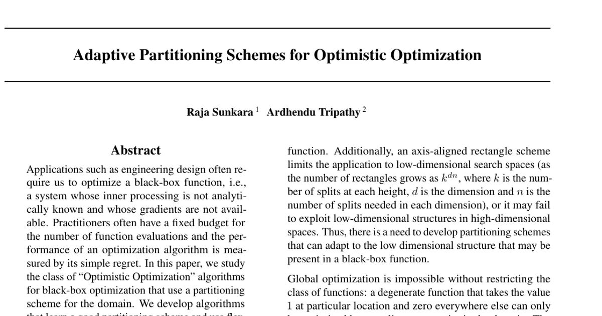
Applications such as engineering design often require us to optimize a black-box function, i.e., a system whose inner processing is not analytically known and whose gradients are not available. Practitioners often have a fixed budget for the number of function evaluations and the performance of an optimization algorithm is measured by its simple regret. In this paper, we study the class of "Optimistic Optimization" algorithms for black-box optimization that use a partitioning scheme for the domain. We develop algorithms that learn a good partitioning scheme and use flexible surrogate models such as neural networks in the optimization procedure. For multi-index functions on an $m$-dimensional subspace within $d$ dimensions, our algorithm attains $\tilde{O}(n^{-β/ d})$ regret, where $β= 1 + \frac{d-m}{2m-1}$, as opposed to $\tilde{O}(n^{-1/d})$ for SequOOL, a state-of-the-art optimistic optimization algorithm. We use our approach to improve the quality of Activation-aware Weight Quantization (AWQ) of the OPT-1.3B model, achieving $\sim10\%$ improvement in performance relative to the best possible unquantized model.