A Unified Framework for Automated Assembly Sequence and Production Line Planning using Graph-based Optimization

AI summary

Overview

• Research area: Manufacturing process planning — specifically Assembly Sequence Planning (ASP) and Production Line Planning (PLP), combining CAD geometry analysis, graph-based optimization, and Mixed-Integer Programming (MIP).
• Technical level: Advanced. The paper assumes familiarity with directed graphs, Degree of Freedom matrices, CAD mesh representations, and mixed-integer optimization.
• Scope: A single open-source Python framework (PyCAALP) that automates assembly sequencing and station time balancing for industrial assemblies, from 3D CAD input to station-level production plans.

What This Paper Is About

Factory planning requires deciding both the order in which parts are joined (assembly sequence) and how those operations are distributed across a fixed number of manufacturing stations (line balancing). Most existing methods treat these as separate problems, and the joint solution space grows explosively — an assembly with 17 joints can produce a directed graph with an upper bound of 1,114,112 edges. The paper presents PyCAALP, a framework that solves both problems together as one weighted graph optimization, adds geometric feasibility checks derived from CAD Degree of Freedom matrices, and uses a deterministic subgraph reduction to keep the optimization solvable for complex assemblies.

Key Contributions

1. A unified formulation of ASP and PLP. The objective is a single weighted sum, J = (1−λ)·C_eng + λ·C_time, where λ ∈ [0,1] is a user-defined factor trading off engineering-constraint quality against station time balance. This lets the user steer the solution between assembly-sequence concerns and line efficiency.

2. Automatic geometric constraint modeling from CAD. Joints, coordinate systems, and 3×4 Degree of Freedom matrices are extracted automatically from STL triangle meshes. Spatial relationships between part pairs are classified as contact, blocking, or free, using the Flexible Collision Library (FCL) for contacts and a PyVista raytracing method for blocking. Degree of Freedom entries are set to zero whenever a tested displacement produces an intersection volume above a tolerance of 0.1 mm³.

3. A deterministic path-guided edge reduction for the MIP. Instead of pruning the directed graph arbitrarily, the framework solves the MIP on a subgraph D′ ⊆ D built from a set of complete, high-quality start-to-end paths, guaranteeing feasibility by construction. Six enumeration strategies based on Yen's k-shortest simple paths (as implemented in NetworkX) are defined and evaluated, including an adaptive strategy that switches from a blended union enumeration to a diverse penalized rerouting once edge growth stalls.

4. An open-source, Python-based implementation. PyCAALP is released at https://github.com/TUM-utg/PyCAALP, using NetworkX for graphs, PyVista, MeshLib, trimesh and FCL for geometry, and PySCIPOpt as the MIP solver.

Main Findings

• Geometric constraints substantially shrink the search space in the tested case. The theoretical upper bound on directed-graph edges is J·2^(J−1) (Eq. 4). For Assembly 2 (15 parts, 17 joints) that upper bound is 1,114,112 edges (≈1.1×10⁶); after constraints, the directed graph retains 134,216 edges. For Assembly 1 (14 parts, 13 joints) the upper bound is 53,248 (≈5.3×10⁴), roughly two orders of magnitude smaller than Assembly 2.

• Full MIP solves are slow for the larger assembly. Solving the full MIP on Assembly 2's 134,216-edge graph to optimality requires between a few minutes and roughly 4.7 h, depending on the time-balancing factor λ (Table 1). The difficulty depends on graph structure, not joint count alone, and is especially affected at higher λ values.

• The reduction preserves feasibility by construction. Because D′ is assembled from complete paths, it always admits a feasible flow, and since D′ ⊆ D, its optimum is an upper bound on the full-graph optimum. The authors state it can never return an infeasible or invalid assembly sequence, at any budget — unlike unstructured pruning that discards low-weight edges and can sever every start-to-end path.

• Reduction reproduces the full-graph optimum exactly or near-exactly at a small fraction of the graph. The abstract reports speedups of up to three orders of magnitude. In the authors' test cases, the reduction becomes beneficial for the 17-joint Assembly 2.

• Enumeration strategy design matters. The paper argues the design question is not whether to keep paths but which paths to enumerate. It reports that bl-union discovers high-quality paths but saturates (additional paths reuse existing edges), while the diverse penalty method grows without bound but can skip high-quality paths — motivating the combined adaptive strategy.

• Two industrial assemblies were used for evaluation. Assembly 1 (14 parts, 13 joints) serves as a correctness baseline and is used to analyze sensitivity to the engineering weights μ and the time-balancing factor λ; Assembly 2 (15 parts, 17 joints) tests geometric constraints and the reduction method.

• Not reported in the provided content: The detailed quantitative results of the reduction study (Section 6.3.2), the sensitivity analysis results for μ and λ, and the full results tables are not included in the truncated text, so no accuracy percentages or per-instance timings beyond the 4.7 h and "up to three orders of magnitude" figures can be stated.

Methodology in Plain English

Step 1 — Pre-processing. CAD models are exported as STL triangle meshes. Parts become nodes and joints become edges in an undirected graph. Attributes (part mass, handling complexity, joint time, tolerance, joining technology) are loaded from a JSON file and normalized. For each joint, a local coordinate system is built as a 4×4 homogeneous transformation matrix from translation and rotation components.

Step 2 — Geometric feasibility. Each pair of parts is classified as contact, blocking, or free. For contact and blocking pairs, the framework mechanically moves one part and measures the resulting intersection volume using MeshLib. If the volume exceeds 0.1 mm³, that direction of motion is marked unavailable. Translations are generated adaptively: for each axis the projected characteristic length of the moved part is scaled by a range factor of 2.0 and split into five equal steps, giving test distances from 0.4 to 2.0 times the characteristic length in both directions. Rotations use six fixed angles (15°, 45°, 75°, 90°, 120°, 150°) in both rotational senses. Because extra tests can only zero further entries, the procedure cannot admit a geometrically infeasible operation, and it needs no per-assembly tuning.

Step 3 — Sequence graph generation. A layered directed graph is built by removing one joint at a time, starting from the fully connected assembled part. Each layer equals one joint addition, so the number of layers equals the number of joints plus one. Edge weights combine technology, handling, and tolerance contributions with user weights μ_tech + μ_hand + μ_tol = 1, divided by the current layer number so that risky operations (technology changes, high handling requirements, tight tolerances) are pushed to later stages. Single-Piece Flow is enforced by requiring the remaining assembly graph to form a single subassembly at each step. An optional collision check uses the Degree of Freedom matrices, transformed into the reference frame of the newly added joint, and compares the count of available translational freedoms using the L₀ norm.

Step 4 — Line planning. A MIP assigns each joint to a station. Binary variables x select edges (the sequence), y assign graph layers to phases, and z assign operations to phases; a continuous variable α tracks the maximum phase time. Constraints enforce flow conservation, one phase per layer, monotonic phase ordering, one phase per operation, and the coupling between x, y, and z. A pre-calculated factor c equalizes the magnitude of the assembly and line-planning terms so λ meaningfully controls the trade-off. The MIP is solved with PySCIPOpt.

Step 5 — Reduction (optional). For large cases, the MIP runs on a subgraph grown by enumerating complete paths until a user-defined percentage of the original edge set is reached — a percentage budget is preferred over a fixed path count because it is comparable across assemblies.

Why This Matters

• Research impact: The paper links two planning problems that are usually solved separately, and it proposes a reduction scheme with a formal feasibility guarantee (D′ ⊆ D, built from complete paths), which the authors contrast explicitly with unstructured edge pruning that can leave the MIP infeasible. It also contributes a CAD-derived method for building Degree of Freedom matrices, including adaptive translation test scales.

• Real-world applications:

  • Automotive and emissions-control assembly lines, where a fixed number of stations must be loaded evenly.
  • Welded structures and metal-forming assemblies, where joining technology (the paper's example uses "MAG" vs "MAG2" welding) and weld length drive operation times.
  • High-mix or customized production, where planning must be repeated quickly when product or constraint data changes.
  • Research and teaching environments needing an openly available, inspectable planning pipeline rather than a black-box tool.

• Industry relevance: The framework connects directly to CAD data that manufacturers already possess but underuse, runs in Python — described by the authors as the standard language for engineering integration — and supports re-running assembly planning and time balancing while pre-processing only once. The authors note that deep-learning approaches often need large task-specific and company-dependent labeled datasets, limiting generalization in highly customized environments, whereas this framework relies on geometry and user-defined engineering weights.

Future Directions

• Full empirical validation of the reduction strategies. The paper states that how closely the reduced optimum tracks the full-graph optimum is assessed empirically in Section 6.3.2; the reported results are not present in the provided content, leaving open how each of the six enumeration strategies performs across assemblies, λ values, and subgraph budgets.
• Extending geometric constraint extraction to assemblies without CAD-derived Degree of Freedom matrices. The collision check is optional and available only where these matrices exist; for Assembly 1 the step is skipped.
• Scaling and tractability of the full MIP. The authors note that difficulty depends on graph structure rather than joint count alone, particularly at higher λ values, raising the question of how the approach behaves beyond 17-joint assemblies.
• Calibration of the heuristic surrogates. The blended enumeration uses a path-additive phase-misalignment proxy rather than the true objective (which uses the maximum phase time α), and the equalizing factor c is pre-calculated from the standalone optimal solutions — both are approximations whose effect on solution quality remains to be characterized.

Target Audience

Researchers and practitioners in manufacturing systems engineering, computer-aided process planning, and production line design; industrial engineers working with CAD-driven assembly planning; and operations researchers interested in MIP formulations for line balancing with graph-reduction techniques. Undergraduate readers would need background in graph optimization and mixed-integer programming to follow the MIP constraints and reduction arguments.

Authors’ abstract

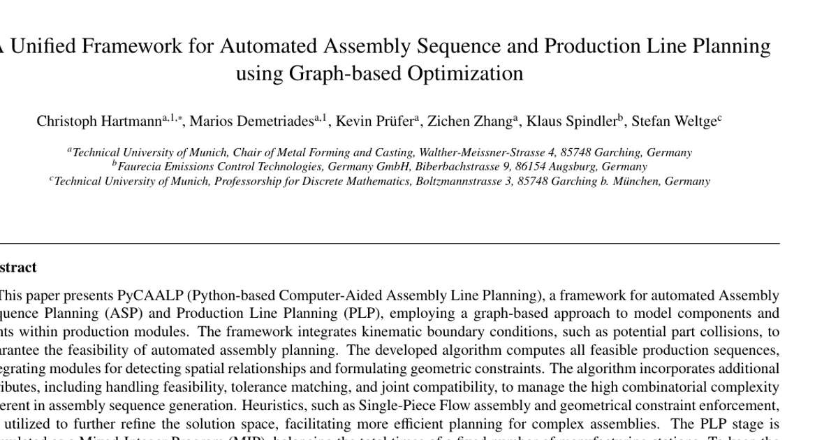
This paper presents PyCAALP (Python-based Computer-Aided Assembly Line Planning), a framework for automated Assembly Sequence Planning (ASP) and Production Line Planning (PLP), employing a graph-based approach to model components and joints within production modules. The framework integrates kinematic boundary conditions, such as potential part collisions, to guarantee the feasibility of automated assembly planning. The developed algorithm computes all feasible production sequences, integrating modules for detecting spatial relationships and formulating geometric constraints. The algorithm incorporates additional attributes, including handling feasibility, tolerance matching, and joint compatibility, to manage the high combinatorial complexity inherent in assembly sequence generation. Heuristics, such as Single-Piece Flow assembly and geometrical constraint enforcement, are utilized to further refine the solution space, facilitating more efficient planning for complex assemblies. The PLP stage is formulated as a Mixed-Integer Program (MIP), balancing the total times of a fixed number of manufacturing stations. To keep the MIP tractable for complex assemblies, a deterministic path-guided reduction solves it on a subgraph assembled from complete, high-quality assembly paths, which preserves feasibility by construction and reproduces the full-graph optimum, exactly or near-exactly, at a small fraction of the directed graph and with speedups of up to three orders of magnitude. Furthermore, the framework enables customization of engineering constraints and supports a flexible trade-off between ASP and PLP. The open-source nature of the framework, available at https://github.com/TUM-utg/PyCAALP, promotes further collaboration and adoption in both industrial and production research applications.