Technical Deep Dives
Retrieval-Augmented Generation: Architecture and Best Practices
The complete guide to building and optimizing RAG systems. Covers chunking strategies, embedding selection, retrieval algorithms, re-ranking, and production deployment.

Gabriele Masetti ·
Why RAG exists, and where it breaks
A model with perfect reasoning and zero access to your data is useless for most enterprise questions. Retrieval-augmented generation exists to close that gap: instead of retraining or fine-tuning a model every time your knowledge base changes, you fetch relevant passages at query time and hand them to the model as context.
The idea traces back to Lewis et al.'s 2020 NeurIPS paper "Retrieval-Augmented Generation for Knowledge-Intensive NLP Tasks," which combined a dense passage retriever with a sequence-to-sequence generator and showed it beat pure parametric models on open-domain QA. Five years later, the core idea is unchanged, but the engineering around it has grown into its own discipline, with distinct failure modes at every stage: ingestion, chunking, embedding, indexing, retrieval, reranking, and generation.
Most teams that say "our RAG system doesn't work" have actually diagnosed nothing — the failure could be in any of those seven stages, and each has a different fix. The piece walks the pipeline stage by stage, with the specific techniques and numbers that separate a demo from a production system.
The ingestion and chunking layer
Chunking decides what unit of text gets embedded and retrieved. Get it wrong and no amount of downstream cleverness recovers the lost information.
Fixed-size chunking (e.g., 512 tokens with 10-15% overlap) is the default in LangChain's RecursiveCharacterTextSplitter and LlamaIndex's SentenceSplitter. It's cheap and predictable, but it cuts through sentences, tables, and logical sections indiscriminately. A financial 10-Q chunked at a fixed boundary will happily split a revenue table from its column headers.
Semantic chunking groups sentences by embedding similarity, breaking where adjacent sentences diverge past a threshold. It respects topic boundaries better but costs an embedding pass just to decide where to cut, and it can produce wildly uneven chunk sizes.
Structure-aware chunking uses the document's own markup — markdown headers, HTML tags, PDF layout blocks — as chunk boundaries. Structure-aware chunking is usually the highest-leverage option for structured corpora (docs sites, contracts, SEC filings) because it preserves the author's own semantic units.
The deeper problem all three share is that an isolated chunk loses the context of the document it came from. A chunk that just says "Revenue grew 12% in the segment" is useless without knowing which company, which quarter, which segment. Two techniques attack this directly:
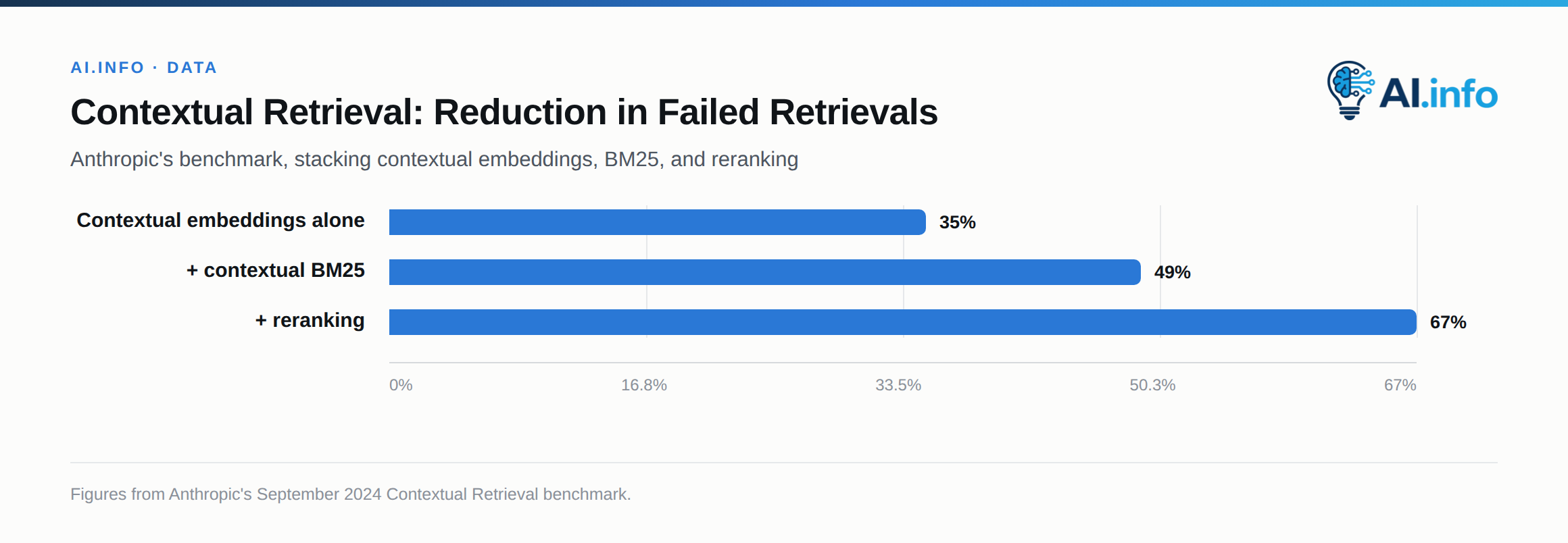
- Contextual Retrieval, published by Anthropic in September 2024, prepends a short LLM-generated summary to each chunk before embedding — something like "This chunk is from Acme Corp's Q3 2024 10-Q, discussing segment revenue for the cloud division" — and indexes the enriched chunk in both the vector store and a BM25 index. Anthropic's own benchmarks reported a 35% reduction in failed retrievals from contextual embeddings alone, 49% when combined with contextual BM25, and 67% when a reranking step was added on top. Because the context-generation prompt is nearly identical across chunks of the same document, it's a natural fit for prompt caching, which keeps the added cost low.
- Late chunking, introduced by Jina AI researchers (Günther et al., arXiv:2409.04701, September 2024) inverts the usual order: embed the entire document first with a long-context embedding model, then pool the token-level embeddings within each chunk boundary afterward. Because the token embeddings were computed with full-document attention, each resulting chunk embedding carries information about the rest of the document, without any added LLM calls. It requires an embedding model with a long context window — Jina first shipped it in
jina-embeddings-v3.
Both approaches are answers to the same root cause: chunk-level embeddings are locally accurate but globally blind.
Embedding models: picking the encoder
The embedding model determines what "similar" means in your vector space, and the field has moved fast enough that a model chosen in 2024 is probably not your best option in 2026. On the MTEB (Massive Text Embedding Benchmark) leaderboard, OpenAI's text-embedding-3-large — the workhorse for a huge share of production RAG systems since its January 2024 release — is still OpenAI's newest as of September 2026, with text-embedding-ada-002 marked legacy behind it. It has been passed on most retrieval benchmarks by newer entrants: Voyage AI's voyage-3-large, Google's Gemini Embedding models, and open-weight models like Alibaba's Qwen3-Embedding series and Jina's v5 line, whose omni variants have since May 2026 embedded text, images, audio, video and PDFs into one shared space.
Qwen3-Embedding-8B led the MTEB multilingual leaderboard in mid-2025 with a score of 70.58, and it carries an open licence, which matters if data residency forces you to self-host. Positions at the top of that board turn over every few months and the board now ranks more than a thousand models, so read any specific ranking — that one included — as a date-stamped snapshot rather than a standing recommendation.
The practical decision isn't "which model tops the leaderboard" — MTEB aggregates across tasks that may not resemble your retrieval workload. It's:
- Does the model's training distribution resemble your domain (legal, code, biomedical, multilingual)?
- What's the maximum input length, and does it exceed your chunk size with room to spare?
- Is the vector dimensionality (and therefore your index's memory footprint) acceptable at your corpus scale — Matryoshka-trained models like
text-embedding-3-largelet you truncate dimensions with graceful degradation, which is a real lever for cost control. - Can you afford API latency and per-token cost at ingestion volume, or do you need a self-hosted encoder?
Re-embed your evaluation set whenever you're considering a switch — embedding model changes are not backward compatible, and mixing vectors from two different models in one index silently corrupts nearest-neighbor search.
Storing and searching the vectors
Once you have embeddings, you need an index that returns approximate nearest neighbors fast. Two index families dominate:
- HNSW (Hierarchical Navigable Small World graphs) builds a multi-layer graph where each vector connects to its nearest neighbors; search starts at a sparse top layer and descends into denser layers, typically touching only a few hundred nodes to find near-optimal matches among millions of vectors. It's the default in pgvector, Weaviate, and Qdrant, offering strong recall (often above 95%) at low latency, at the cost of higher memory usage and slower index builds than alternatives.
- IVF (inverted file index) with product quantization (PQ), the combination FAISS made popular, clusters vectors into Voronoi cells at index time and restricts search to the nearest cell(s), while PQ compresses each vector into a small code to cut memory — Meta's own guidance suggests roughly a 1:1000 cluster-to-vector ratio with 8-16 byte PQ codes for production use. The trade is some recall for a dramatically lower memory footprint, which matters once you're indexing hundreds of millions of vectors.
On infrastructure choice: pgvector turns Postgres into a vector store, which is attractive if you already run Postgres and want vector search, metadata filtering, and transactional writes in one system rather than syncing two databases. Recent pgvector releases have substantially closed the performance gap with dedicated vector databases — HNSW index builds got dramatically faster in the 0.7.0 release. FAISS is a library, not a service — you embed it into your own retrieval code and manage persistence yourself, which suits teams that want full control over indexing parameters. Managed vector databases (Pinecone, Weaviate, Qdrant, Milvus) trade that control for operational simplicity: replication, horizontal scaling, and filtering are handled for you.
A minimal FAISS index for a few hundred thousand chunks looks like this:
import faiss
import numpy as np

dim = 1024  # matches your embedding model's output dimension
quantizer = faiss.IndexFlatIP(dim)
index = faiss.IndexIVFPQ(quantizer, dim, 1024, 16, 8)  # 1024 clusters, 16-byte codes
index.train(training_vectors)   # a representative sample, e.g. 50-100k vectors
index.add(all_vectors)
index.nprobe = 16  # cells searched at query time; trade recall for speed
distances, ids = index.search(query_vector, k=20)
Hybrid search: don't abandon keyword matching
Pure dense retrieval systematically underperforms on exact-match queries: product SKUs, error codes, legal citations, rare proper nouns. A dense encoder trained to capture semantic similarity has no strong incentive to distinguish "invoice #48213" from "invoice #48214" — they're semantically near-identical but you need the exact one. Hence production RAG systems almost universally run a lexical retriever (BM25, or its learned-sparse cousin SPLADE) alongside the dense retriever and fuse the two ranked lists.
Reciprocal Rank Fusion (RRF) is the standard fusion method precisely because it sidesteps the score-normalization problem: BM25 scores are unbounded and corpus-dependent, cosine similarities are bounded between -1 and 1, and there's no principled way to combine them directly. RRF ignores score magnitude and combines documents purely by rank position, using the formula:
RRF_score(d) = Σ 1 / (k + rank_i(d))
summed across each retriever i, with k typically set around 60. Hybrid retrieval with RRF consistently beats either retriever alone on NDCG in published benchmarks, and it's supported natively in Elasticsearch, OpenSearch, Weaviate, and Qdrant.
Reranking: the second-pass filter
Retrieval and reranking solve different problems. A bi-encoder (the architecture behind most embedding models) encodes queries and documents independently, which is what makes it fast enough to search millions of vectors — but that independence also throws away query-document interaction signal. A cross-encoder reranker takes the query and a candidate document together as a single input and produces one relevance score per pair, capturing interactions a bi-encoder can't, at the cost of being far too slow to run over an entire corpus.
The standard pattern: retrieve a wide candidate set (50-100 chunks) with the cheap bi-encoder/hybrid step, then rerank that shortlist down to the 5-10 chunks that actually go into the prompt. Cohere's managed line is now rerank-v4.0-pro, a multilingual model tuned for quality across English, non-English and semi-structured JSON documents, with rerank-v4.0-fast as the low-latency, high-throughput sibling; rerank-v3.5 and the v3.0 English and multilingual models are still served. BAAI's open-source bge-reranker-v2-m3 (Apache 2.0, 100+ languages) still scores a shortlist in 50-100ms on a GPU. Jina moved to jina-reranker-v3.5 on 27 July 2026 — 0.6 billion parameters, a 131K-token context, listwise scoring — and kept the October 2025 v3 published alongside it.
Reranking is the stage Anthropic's contextual retrieval benchmark showed the largest marginal gain from — reranking on top of contextual embeddings and BM25 pushed the failed-retrieval reduction from 49% to 67%.
| Reranker | Type | Notes |
|---|---|---|
| Cohere rerank-v4.0-pro / -fast | Managed cross-encoder | Pro for quality, fast for throughput; multilingual, handles JSON |
| BAAI bge-reranker-v2-m3 | Open-source, Apache 2.0 | 50-100ms on GPU, 100+ languages |
| Jina jina-reranker-v3.5 | Open, listwise scoring | 131K-token context, 0.6B parameters (July 2026) |
Beyond naive RAG: graph and self-correcting architectures
Standard RAG answers questions where the relevant fact lives in one or two retrievable chunks. It fails on questions that require synthesizing across an entire corpus — "what are the major themes in this collection of documents" has no single passage that answers it.
GraphRAG, from Microsoft Research (Edge et al., "From Local to Global: A Graph RAG Approach to Query-Focused Summarization," arXiv:2404.16130, April 2024), addresses this by building a knowledge graph over the corpus: extracting entities and relationships with an LLM, clustering the graph into hierarchical communities using the Leiden algorithm, and pre-generating community summaries. At query time, a "global search" query is answered by synthesizing across relevant community summaries rather than searching raw chunks.
Microsoft reported higher comprehensiveness and diversity in generated answers compared to naive RAG, at the cost of a much more expensive and complex indexing pipeline — full corpus graph extraction is not something you re-run casually.
Two other architectures address retrieval quality directly rather than corpus-level synthesis:
- Self-RAG (Asai et al., 2023, arXiv:2310.11511) fine-tunes a language model to emit special reflection tokens that decide, inline, whether retrieval is needed for a given query and whether a candidate passage actually supports the generated claim — turning retrieval and self-critique into a learned, integrated behavior rather than a fixed pipeline stage.
- Corrective RAG (CRAG) (arXiv:2401.15884, 2024) adds a lightweight retrieval evaluator that scores retrieved documents' relevance and, when confidence is low, triggers corrective actions — such as falling back to web search or decomposing and recomposing the retrieved passages to strip irrelevant content before generation.
Both are worth adopting selectively: they add latency and complexity, and are best reserved for domains where retrieval failures are costly (legal, medical, financial) rather than applied universally.
Evaluation: measuring the pipeline, not just the answer
The most common mistake in RAG evaluation is only checking whether the final answer looks right. That conflates two independent failure surfaces: did retrieval surface the right passages, and did generation use them faithfully? RAGAS, an open-source Python evaluation framework, is built around exactly this separation, using an LLM-as-judge to score along several axes:
- Faithfulness — the fraction of claims in the generated answer that are actually supported by the retrieved context (catches hallucination even when retrieval was correct).
- Answer relevancy — how directly the generated answer addresses the original query (catches cases where the model latches onto retrieved-but-tangential content).
- Context precision — whether the relevant chunks were ranked near the top of what was retrieved.
- Context recall — whether retrieval found all the information needed to answer completely, measured against a reference answer.
Running these four metrics separately turns a vague "the RAG system feels off" into an actionable diagnosis: low context recall means fix chunking or the retriever; high context recall with low faithfulness means the generation step is ignoring or contradicting its own retrieved context, which is a prompting problem, not a retrieval problem.
Failure modes worth planning for
Even a well-built pipeline degrades in predictable ways:
- Lost in the middle. Liu et al. (Stanford, arXiv:2307.03172, 2023) showed that LLM accuracy on long-context tasks is highest when the relevant passage sits at the very start or end of the context window, and drops measurably when it's buried in the middle — regardless of context window size. Retrieval order therefore matters even after the right chunks are found: put your highest-confidence passages first and last, not lumped in the middle of a ten-chunk stuff.
- Retrieval-generation mismatch. The retriever surfaces technically relevant but insufficient chunks (a table without its caption, a clause without the definitions section it depends on), and the model either hallucinates the gap or gives an underspecified answer.
- Chunk boundary amputation. A chunk that ends mid-sentence or mid-table loses the very information a query is looking for — a strong argument for structure-aware or late chunking over naive fixed-size splitting.
- Stale indexes. Vector stores don't know a source document changed unless your ingestion pipeline explicitly re-embeds and re-indexes it; silent staleness is one of the most common causes of "the bot is telling people outdated policy" incidents in production.
RAG versus long context: not a replacement
As context windows have grown into the hundreds of thousands of tokens, a recurring question is whether RAG is still necessary — why retrieve at all if you can just stuff the whole corpus into the prompt? Two things push back on that. First, the lost-in-the-middle effect means a bigger context window doesn't guarantee the model actually uses everything in it; retrieval is a form of attention curation, not just a workaround for a small window.
Second, cost and latency scale with tokens processed regardless of context limit — retrieving 10 relevant chunks out of a million-document corpus is cheaper and faster than reprocessing the whole corpus per query, and it's the only approach that scales past what fits in any context window at all. In practice, the two are complementary: long context reduces how aggressively you need to chunk and how many passages you need to retrieve, but it doesn't eliminate the need to first find the relevant subset of a large corpus.
Building the pipeline that survives production
The teams that get RAG working reliably converge on a few habits: they evaluate retrieval and generation separately rather than eyeballing final answers, they hybridize BM25 and dense retrieval rather than betting everything on embeddings, they rerank before generation rather than trusting raw vector similarity, and they treat chunking as a first-class design decision tied to document structure rather than an afterthought default.
None of this is exotic — it's disciplined application of techniques that are now well-documented and, increasingly, well-benchmarked. The gap between a RAG demo and a RAG system that survives a year of real user queries is almost entirely in how rigorously each of these stages gets tested against the failure modes above, not in finding some undiscovered trick.