Technical Deep Dives
Mixture of Experts: Scaling AI Models Efficiently
How Mixture of Experts lets a model carry trillions of parameters while activating a few percent of them per token — the routing, load balancing and memory maths behind DeepSeek-V4, Kimi K3 and GLM-5.3.

Gabriele Masetti ·
Sparse Activation: The Core Idea
Standard dense transformers apply the same feed-forward network (FFN) to every token, so parameter count and per-token compute rise together — widen the FFN and you pay for that width on every single token that passes through it. Mixture of Experts (MoE) breaks that coupling. Instead of one FFN per layer, an MoE layer holds many parallel FFNs, called experts, plus a small router that decides which subset of experts processes each token.
Total parameter count scales with the number of experts, but per-token compute scales only with however many experts are actually selected. A model can carry hundreds of billions of parameters while doing the arithmetic work of a model an order of magnitude smaller.
The idea of routing inputs to specialized sub-networks goes back to Jacobs, Jordan, Nowlan, and Hinton's 1991 work on adaptive mixtures of local experts, but it became practical for large-scale language modeling only once Google worked out how to route, balance, and train sparse expert layers across thousands of accelerators. Two papers set the modern template: GShard (Lepikhin et al., 2020) and Switch Transformer (Fedus, Zoph, and Shazeer, 2021).
The Router: Gating and Top-k Selection
Every MoE layer replaces (or augments) a dense FFN with N expert FFNs and a router. For a token with hidden representation x, the router computes logits with a learned projection, logits = x · W_g, and a softmax over those logits produces a probability distribution across the N experts. The router keeps only the top-k values (commonly k=1 or k=2), zeroes out the rest, and renormalizes the retained probabilities into gate weights g_i. The layer's output is a weighted sum over just the selected experts:
y = Σ (i in top-k) g_i · E_i(x)
The top-k truncation is where sparsity actually comes from. If k equaled N, every expert would run on every token — a dense mixture with zero compute savings, only extra parameters. Restricting each token to a small, fixed number of experts, regardless of how many experts exist in total, is what keeps per-token FLOPs constant as the expert count grows.
Switch Transformer's central simplification was pushing k down to 1: a single expert handles each token. Fedus, Zoph, and Shazeer showed this "switch routing" preserved model quality while cutting router computation and cross-device communication relative to GShard's top-2 default, and it let them scale T5-based encoder-decoder models beyond a trillion parameters while training parts of the network in bfloat16. Their paper reports up to a 7x improvement in pre-training speed over T5-Base and T5-Large baselines at matched compute.
GShard, which predates Switch Transformer, used top-2 routing: the top-scoring expert is always dispatched, and a second expert is chosen stochastically, with probability proportional to its own gate weight — a "random routing" step meant to spread load rather than always dispatching the same runner-up. Google used GShard's automatic operator sharding to scale a multilingual machine-translation Transformer with sparsely-gated MoE layers beyond 600 billion parameters, training it on 2,048 TPU v3 accelerators in four days — a result that demonstrated MoE sharding could be handled largely by compiler annotations rather than hand-written parallelism code.
| System | Total params | Experts (top-k) | Routing innovation |
|---|---|---|---|
| GShard | 600B+ | top-2 | Stochastic second-expert routing |
| Switch Transformer | 1T+ | top-1 | Single-expert routing, up to 7x pretraining speedup |
| DeepSeek-V3 | 671B | 256 (top-8) | Auxiliary-loss-free load balancing |
| GLM-5.3 | 753B | 256 (top-8) + 1 shared | The same 256/top-8 shape, five years after GShard |
| Kimi K3 | 2.8T | 896 (top-16) + 2 shared | Granularity pushed to nearly 900 experts |
Load Balancing: Why Routers Need a Leash
A naive router collapses under its own dynamics: once a few experts get slightly better gradients early in training, they receive more tokens, get more updates, and become even more attractive to the router — a rich-get-richer feedback loop that leaves most experts undertrained while a handful become bottlenecks. Because compute is provisioned for each expert ahead of time as a fixed capacity, overloaded experts also start dropping tokens once they exceed it:
capacity = (tokens_per_batch / num_experts) × capacity_factor
A capacity factor of 1.0 gives every expert exactly its even share of tokens; Switch Transformer found that a factor around 1.25 — 25% headroom above the nominal allotment — kept the token drop rate below 1% without materially increasing memory or communication overhead. Tokens that arrive after an expert is full are dropped and pass through the layer via a residual connection instead, which is a real, measurable quality cost that grows with how imbalanced routing becomes.
The standard fix for the underlying imbalance is an auxiliary load-balancing loss added to the training objective. The Switch Transformer/GShard formulation computes, per batch, the fraction of tokens routed to each expert (f_i) and the average router probability mass assigned to that expert (P_i), then penalizes their dot product summed across experts:
L_aux = α · N · Σ_i f_i · P_i
The term is minimized when tokens and router probability mass are spread evenly across all N experts; the multiplication by N keeps its scale roughly independent of expert count, and α is a small coefficient trading load balance against task loss.
DeepSeek-V3 took a different route to the same goal: an auxiliary-loss-free balancing strategy. Rather than adding a competing gradient term to the loss, it adds a dynamic bias to each expert's routing score before top-k selection and adjusts that bias after each step based on how over- or under-utilized the expert recently was — nudging traffic toward underused experts without a secondary loss term fighting the primary language-modeling objective.
The Architecture Ledger: Real Deployed MoE Models
Mixtral 8x7B, described in Mistral AI's "Mixtral of Experts" paper, is the model that made sparse MoE mainstream outside research labs. Each transformer layer replaces its FFN with 8 experts and a router that selects the top 2 per token. The model holds about 46.7B total parameters, but because only 2 of 8 experts activate per token, a forward pass costs roughly what a ~13B dense model would cost. Mistral reported that Mixtral matched or beat Llama 2 70B and GPT-3.5 on most benchmarks despite that much smaller active-parameter footprint. Both comparison points have since been retired; the claim is a museum label now, but it moved sparse MoE out of research labs and into products.
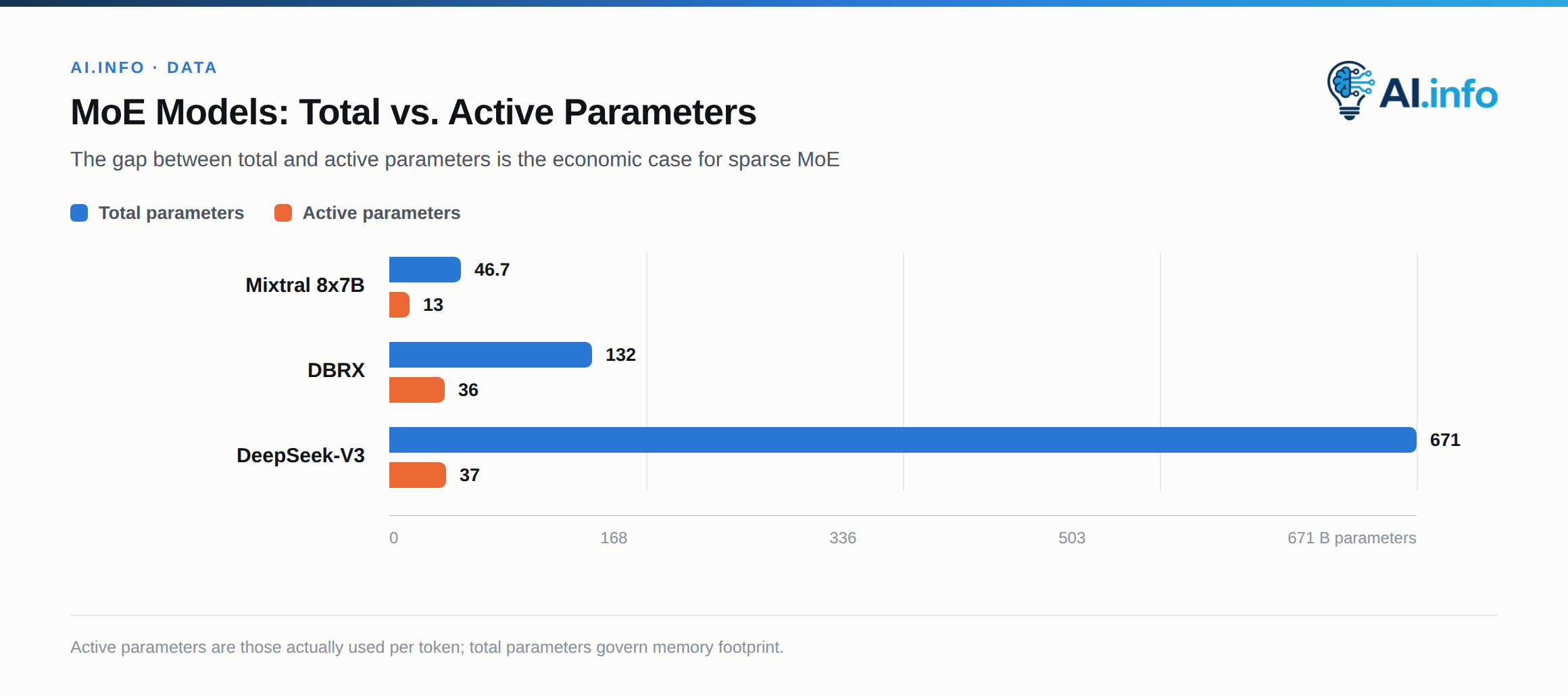
DeepSeek-MoE and DeepSeek-V3 pushed granularity further. Instead of a handful of large experts, DeepSeek's architecture uses fine-grained expert segmentation — splitting the FFN budget into many smaller experts — and designates a subset as shared experts that are always active for every token, isolating common knowledge (grammar, general syntax) from the specialized knowledge that routed experts capture. DeepSeek-V3 scales this to 671B total parameters across 256 routed experts (top-8 selected per token) plus shared experts, activating about 37B parameters per token.
It was pretrained on 14.8 trillion tokens and, according to DeepSeek's technical report, required roughly 2.79 million H800 GPU hours for the full training run — a figure widely cited as evidence that well-engineered MoE training can be dramatically cheaper than dense training at comparable quality.
DeepSeek has since moved two generations past it. V4 was previewed on 24 April 2026: V4-Pro at 1.6 trillion total parameters with 49 billion active, V4-Flash at 284 billion with 13 billion, both MIT-licensed with a one-million-token default context. V4-Pro's model card reports more than 32 trillion pretraining tokens and 80.6 percent on SWE-bench Verified.
Grok-1, released by xAI under an Apache 2.0 license in March 2024 after its pretraining concluded in October 2023, is a 314B-parameter MoE with 8 experts, 2 of which (25%) activate per token — architecturally close to Mixtral's 8-choose-2 pattern but at roughly seven times the total parameter count. At the time of release it was described as the largest openly released MoE model.
DBRX, released by Databricks in March 2024, took granularity in the opposite direction from Mixtral: 16 experts with 4 selected per token, rather than 8-choose-2, which yields many more possible expert combinations for a given token than a coarser design does. DBRX totals 132B parameters with 36B active, and was pretrained on 12 trillion tokens.
The 2026 open-weight frontier moved the design points on. Moonshot AI's Kimi K3, announced 16 July 2026, carries 2.8 trillion total parameters and activates about 104 billion per token, routing each to 16 of 896 experts plus two shared — the largest open-weight release to date. Z.ai's GLM-5.3, open-weighted in August 2026, is a 753-billion-parameter model with 256 routed experts, top-8 selection and one shared expert. Z.ai publishes no active-parameter count; Artificial Analysis puts it at about 40 billion. Alibaba's Qwen3.8-Max, released 3 August 2026 and conditionally open-weighted 12 August as Qwen3.8-2.4T-A95B, is 2.4 trillion total, roughly 95 billion active.
Across all of these a pattern holds: every one uses some variant of learned top-k routing with an explicit load-balancing mechanism, evidence that the GShard/Switch Transformer recipe generalized well beyond Google's original experiments. What changed is how sparse they are. The 2023-24 cohort clustered between about 1:4 and 1:18 active-to-total; the 2026 cohort runs from roughly 1:19 (GLM-5.3) to 1:33 (DeepSeek-V4-Pro), Kimi K3 at about 1:27. Sparsity roughly doubled in two years, and expert counts grew three- to four-fold.
Why This Decouples Parameters from FLOPs
The efficiency argument separates two things dense scaling bundles together: representational capacity and computational cost. In a dense transformer, adding parameters to the FFN means every token pays for those parameters on every forward pass, so capacity and FLOPs scale in lockstep. In an MoE layer, adding experts increases capacity — more distinct FFN subnetworks the model can specialize into — without touching the FLOPs of a token that only visits k of them. Doubling the expert count while holding k fixed roughly doubles total parameters but leaves per-token compute unchanged.
That is why MoE papers report both total and active parameter counts as separate headline numbers. Total parameters govern memory footprint and, empirically, how much the model can specialize and how low its held-out loss can go at a given training-compute budget. Active parameters govern inference latency, serving throughput, and the FLOPs spent per training token. A well-trained MoE model tends to approach the quality of a dense model whose size matches its total parameter count, while running inference at a cost closer to its active-parameter count — that gap between the two numbers is the entire economic case for the architecture.
Inference and Memory: Where the Bill Comes Due
The FLOPs savings are real, but they come with a memory bill that dense scaling doesn't have to pay. Every expert's weights have to sit somewhere accessible, typically in GPU HBM, regardless of whether that expert is used on a given forward pass, because you don't know in advance which experts a batch of tokens will route to. A 671B-parameter MoE model with 37B active parameters still needs enough aggregate memory to hold all 671B parameters, not 37B, even though only 37B worth of compute happens per token. That inverts the usual accelerator bottleneck: MoE inference is compute-light and memory-heavy. Kimi K3 shipped as a native four-bit checkpoint, and 2.8 trillion parameters at roughly half a byte each is about 1.4TB of weights before any KV cache — a multi-node deployment, not a single-server problem.
The standard solution is expert parallelism: shard the experts across devices, with each device holding a subset of expert FFNs plus a full copy of the non-expert parameters (attention layers, embeddings, layer norms). During a forward pass, tokens are dispatched over the network to whichever device holds their selected expert, processed there, and the results are gathered back — two all-to-all communication collectives per MoE layer, one scattering tokens to their experts and one gathering results back to the requesting devices.
Because this communication happens at every MoE layer, interconnect bandwidth — NVLink within a node, InfiniBand or similar across nodes — becomes as important to serving throughput as raw compute.
A second, quieter cost is load imbalance at inference time rather than training time. If a batch of real-world requests happens to route heavily toward a small subset of experts — plausible, since routing correlates with content and live traffic isn't distributed like a shuffled training corpus — the devices hosting those experts become stragglers while others sit idle, and end-to-end latency is set by the slowest device rather than the average one.
Systems built for MoE serving, such as Microsoft's DeepSpeed-MoE, address this with techniques including expert-aware placement and communication scheduling designed to reduce the cost of these all-to-all exchanges rather than merely tolerating them.
What This Means for Model Design
For anyone choosing or deploying an MoE model, the two headline numbers answer two different questions. Total parameters tell you what hardware memory footprint to provision, and roughly, how much task diversity and world knowledge the model can encode. Active parameters tell you what latency and throughput to expect and what compute budget was likely spent per training token. Kimi K3 at 2.8T total and 104B active and Mixtral at 46.7B total and 12.9B active are both "MoE," but they sit at opposite ends of the memory-versus-compute curve — sixty times the memory footprint for eight times the per-token compute — and neither number alone describes the real deployment cost.
The granularity choice is itself a design axis. Few large experts selected with a narrow top-k — Mixtral's 8-choose-2, Grok-1's 8-choose-2 — is architecturally simple and keeps the all-to-all dispatch pattern manageable. Many small experts selected with a wider top-k — DeepSeek-V3's and GLM-5.3's 256-choose-8, DBRX's 16-choose-4, Kimi K3's 896-choose-16 — gives the router far more combinatorial specialization to work with and can improve loss at a fixed active-parameter budget, at the cost of more bookkeeping and more distinct destinations for token dispatch.
The auxiliary-loss-free balancing approach DeepSeek-V3 popularized suggests the field is still actively iterating on how to keep that specialization honest without a competing gradient signal fighting the main training objective. Routing and load balancing, more than raw expert count, remain the part of MoE design most likely to keep changing in the models that follow these.